In the interest of faster field calculations lets investigate interpolation techniques. The idea is to pre-calculate a grid of points in space, store those and later when required to calculate the field at a specific point use the pre-calculated values from the grid to approximate the field value at the given point. There are some disadvantages though, for one the approximation is just that, an approximation so precision suffers. There are two basic ways to increase the precision. One is to increase the grid density but this comes with the penalty in memory usage. The other way is to use more sophisticated interpolation algorithms, but these will use more CPU power.
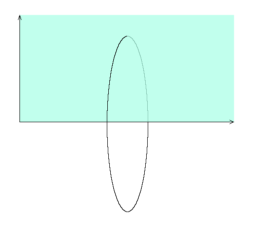
The coils used often have one nice property - they are symmetric. That means the field is defined by two arguments alone: the axial distance from the coil (distance from the coil plane) and the radial distance (distance from the axis of the coil). These two arguments form a plane.
We can calculate a grid of field values on this (bounded) plane and use two-dimensional interpolation algorithms to calculate the field value at any point. The two easiest algorithms to use are nearest neighbour and bilinear interpolation. The fields we calculate are vector fields, that is they have two components. We can interpolate each of those separately using these algorithms.
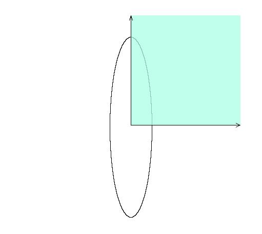
Using this method we can pretty much interpolate coils of any cross-section shape. There is an improvement that can be made here in case the coil cross-section is symmetric. When looking at the b-field we can realize that the field on each side of the coil is very similar, except for the radial component which has an opposite sign. This can be used to optimize the algorithm - we will only need half the memory to get the same grid density. This also works for e-field in ring of charge - the axial component has an opposite sign but same numeric value.
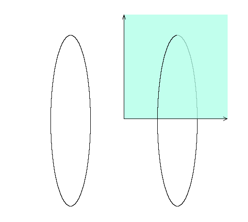
In cube polywell and other applications we deal with coils placed on the same axis. That is in case of cube polywell we have 3 pairs of opposite coils. We can again recognize that the field from those pairs only depends on the axial and radial components of the position in relation to the coils. Also in case of opposite placed coil pair we only need half the plane again as the axial component changes its sign on the opposite sides. In case the coils point the same way and are symmetric no sign changes are even present - we can again use only half the plane. Using coil pairs we can halve memory accesses and interpolation algorithm calculation overhead.
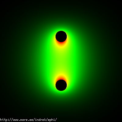
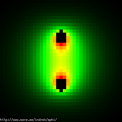
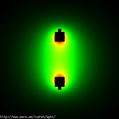
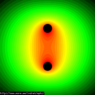
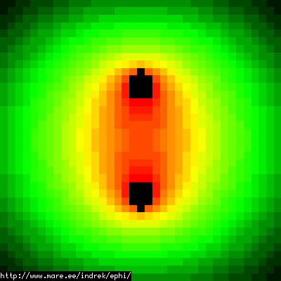
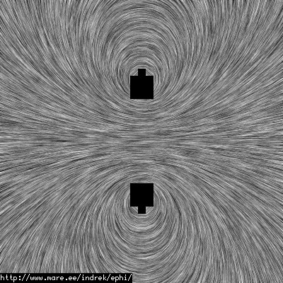
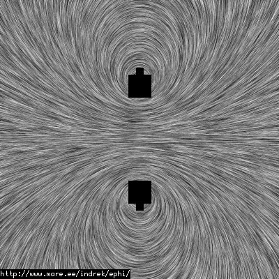
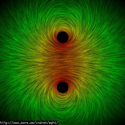
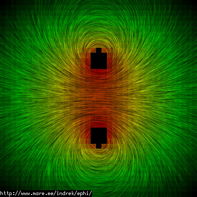
Following are images of a coil field with different calculation techniques. The interpolation grid here is of extreamly low resolution (only 32x32 grid cells - but less visible on these images) to show how well the interpolation algorithms work. You can compare the nearest neighbour here to the bilinear interpolation algorithm.
| Direct calculation | Low resolution nearest neighbour | Low resolution bilinear interpolation |
 |
 |
 |
 |
 |
 |
 |
 |
 |
 |
 |
 |
How dense can a grid be? These days computer memory is very cheap and with 64 bit CPUs we can increase the calculation resolution to the extreams. Lets take an example with following properties: 6GB of RAM and a coil of radius=0.15m and including only the b-field for a plane sized 0.65 x 0.65m. A grid cell will be 2.31795e-05 x 2.31795e-05 large and for single-precision field values we can fit around 28051 x 28051 samples in the 6GB.
Detecting coil body is done here using a separate grid, but this time a bitmap to save on memory.
The speed improvement in ephi gained from bilinear interpolation compared to direct calculation is around 10-12 times. This might seems like a small improvement from direct calculation - the reason is that direct calculation implementation in ephi is very good.
In case both b-field and e-field are interpolated, it probably makes sense to keep the data in one data structure instead of two separate grids. The reason is that the CPU-RAM fetch/pre-fetch/cache performance is probably better when all the data that is used in one go is close together (I haven't really done any benchmarking to confirm this though, so this is a somewhat of a voodoo assessment).
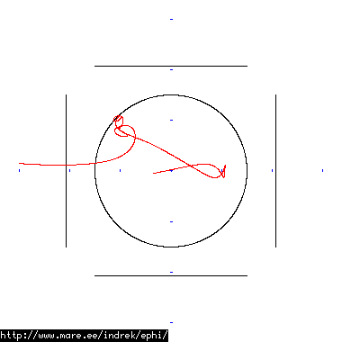
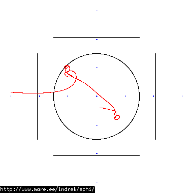
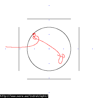
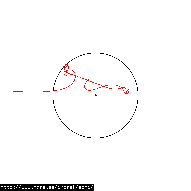
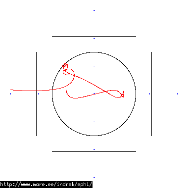
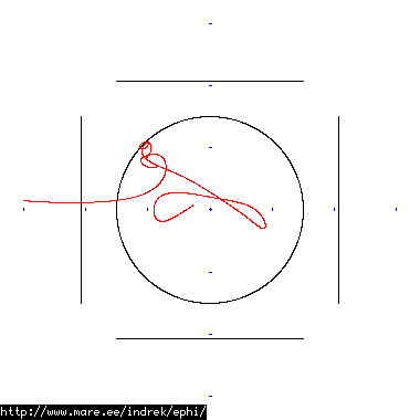
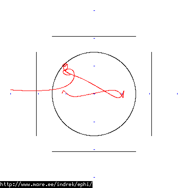
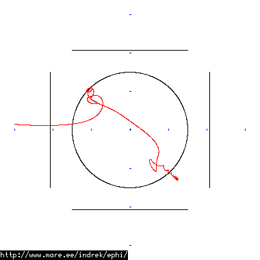
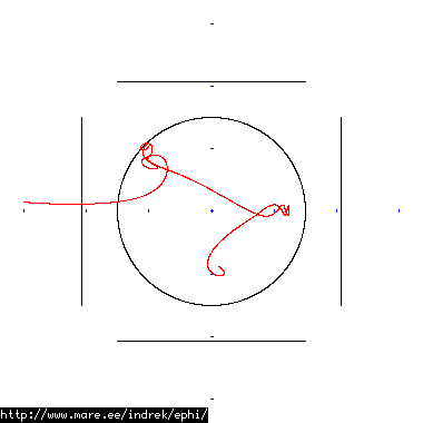
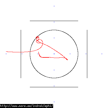
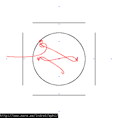
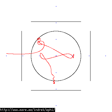
How well does simulating electron paths in ephi work using interpolation? Not terribly well. Here's a test run of a cube polywell electron path simulation from arbitrary starting position. We let it run until the linear interpolation run electron drifts more than a centimeter from direct calculation.
| Direct calculation | Nearest neighbour | Bilinear interpolation | |
| 10 MB 1671 ticks |
 |
 |
 |
| 20 MB 1738 ticks |
 |
 |
 |
| 30 MB 1874 ticks |
 |
 |
 |
| 40 MB 1830 ticks |
 |
 |
 |
| 50 MB 1821 ticks |
 |
 |
 |
| 60 MB 1826 ticks |
 |
 |
 |
| 70 MB 1849 ticks |
 |
 |
 |
| 80 MB 1855 ticks |
 |
 |
 |
| 90 MB 1875 ticks |
 |
 |
 |
| 100 MB 1883 ticks |
 |
 |
 |
| 6000 MB 2296 ticks |
 |
 |
 |
Copyright © 2007 Indrek Mandre