In the polywell the coils are charged using positive high voltage and act as accelerators for the electrons and also provide recirculation for the electrons. As electrons penetrate the magnetic mirror and fly out of the system, the accelerator coils attract them right back in.
So far in my simulations I have used rings of uniform charge to get the effect. Unfortunately electric charge and field does not work that simply. As some parts of the coils are closer to each other the charges from there will flow towards parts that are farther apart. Also the coils are big and round and the charge should intuitevly collect on the side of the coils that is towards the outside of the system.
One way to look at the coils is as of a faraday cage. The textbooks tell us that the electic field within the cage should be 0.
How to get the charge distribution? The standard way is to use the Poisson's equation. We know that the potential on the coils is constant. Also all charge is on the edge of conductor, but almost never within the conductor. The Poisson says:
As we know the potential on the surface of the conductor is constant we can write out a series of linear equations for discrete areas of the conductor surface (the mesh). We get a big system (thousands) of linear equations. If we solve this system we get the charge densities. Once we have that we can calculate the potential and electric fields outside the conductor. Solving of the linear system can be done iteratively (an approximised solution) or exactly (using matrix methods, say Gauss-Jordan elimination, etc). Years ago when I took linear algebra at school I wondered why people bothered with it and if there was any real use for it. There is.
This is the theory but I don't yet have a full understanding on how to implement it. So I did not pursue this method at the start but went with another more primitive mechanism. I divided the surface into points, with connections between adjacent points. I assigned charge to each point and then started moving the charge around according to the electric field at the middle of each connection using the Coulomb law. Now I have to admit this is quite an hackish and slow method of doing things. I promise my next task is to use the proper Poisson equation but on this page I show the results I got with the charge flow method.
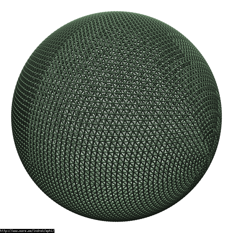
As a benchmark lets start with a simple case of a sphere. This is a sphere with 0.25 meter radius. There are 9823 points and 29463 links in this mesh. The simulation estimates the capacitance of the sphere as 2.79e-11F. The theoretical capacitance is 2.78e-11F. Pretty close match.
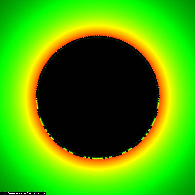
Here's how the electric field of the sphere cross-section looks like, as you can see within the sphere the electric field is close to 0:
For reference here's the color gradient ephi uses:
![]()
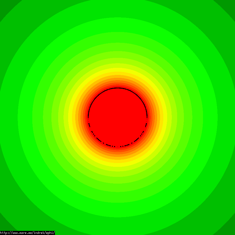
One more thing to look at is the electric potential. Here's a picture of the sphere at 1000 volts, each level indicates change of 50 volts. As you can see everywhere within the sphere the potential is close to 1000V.
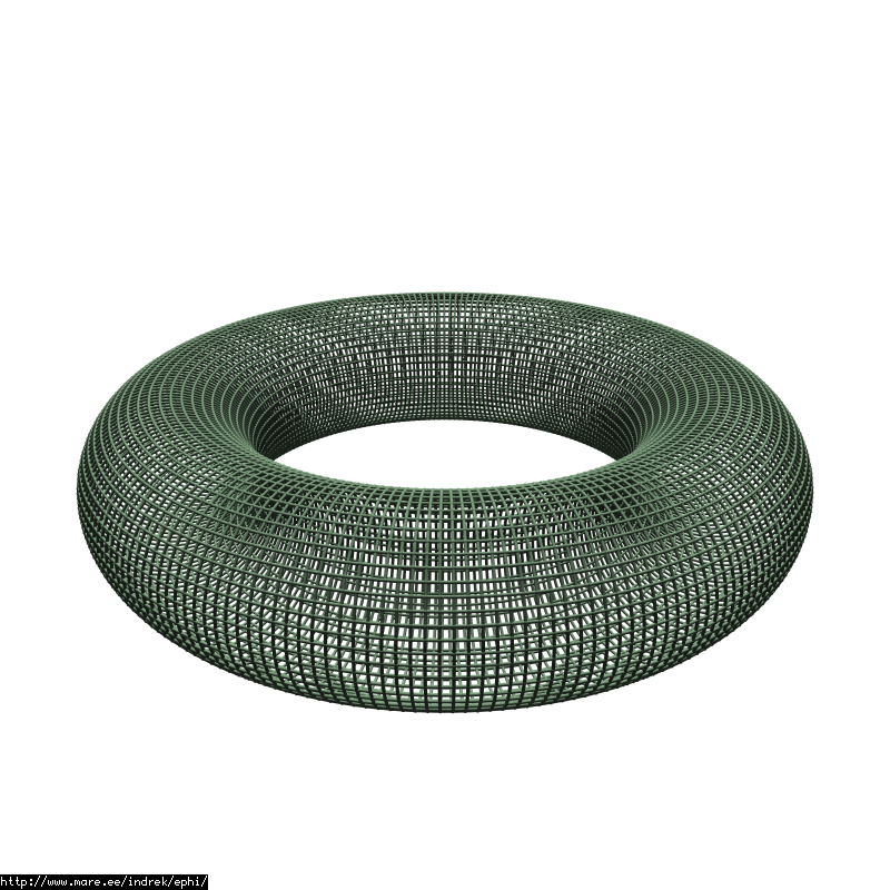
Now I'm reasonably sure my simulation works with most primitive objects. Lets try something more complicated. A torus of radius 0.25m and thickness of 0.125m. This torus consists of 12031 points and 24062 links.
The simulation estimated capacitance is 27.64pF. The theoretical capacitance according to http://www.coe.ufrj.br/~acmq/tesla/capcalc.pdf is 27.59pF. Again a close match. Lets have a look at the efield through the cross-section:
And here's the potential map of the torus at 1000 volts with 50 volt difference between levels.
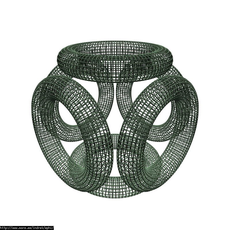
Time to move on to the really interesting stuff. The cube polywell. We construct a cube polywell with 0.15m radius coils that are 0.07m thick and are spaced apart by 0.01m. The simulator estimated capacitance of the device is 30.2pF. The model uses 12240 points and 24480 links.
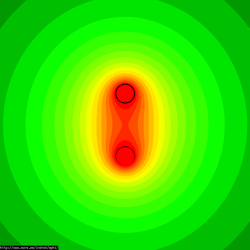
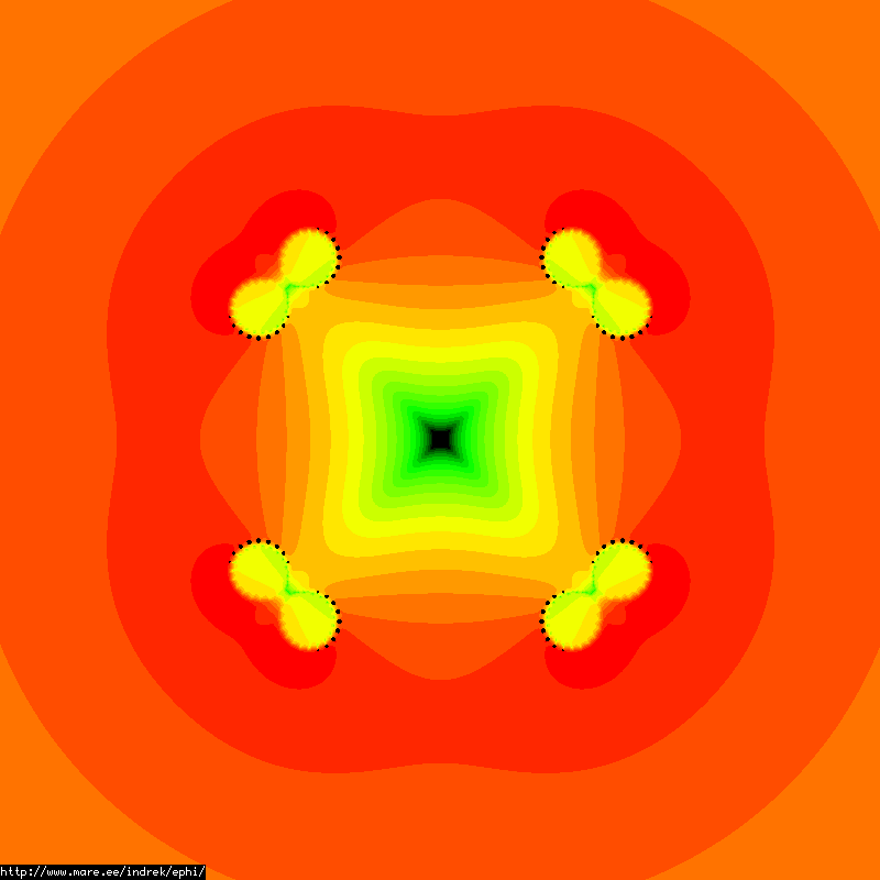
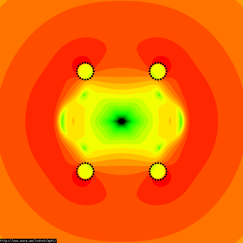
Here's the system charged at 1000 volts and showing potential levels at 50 volt increments:
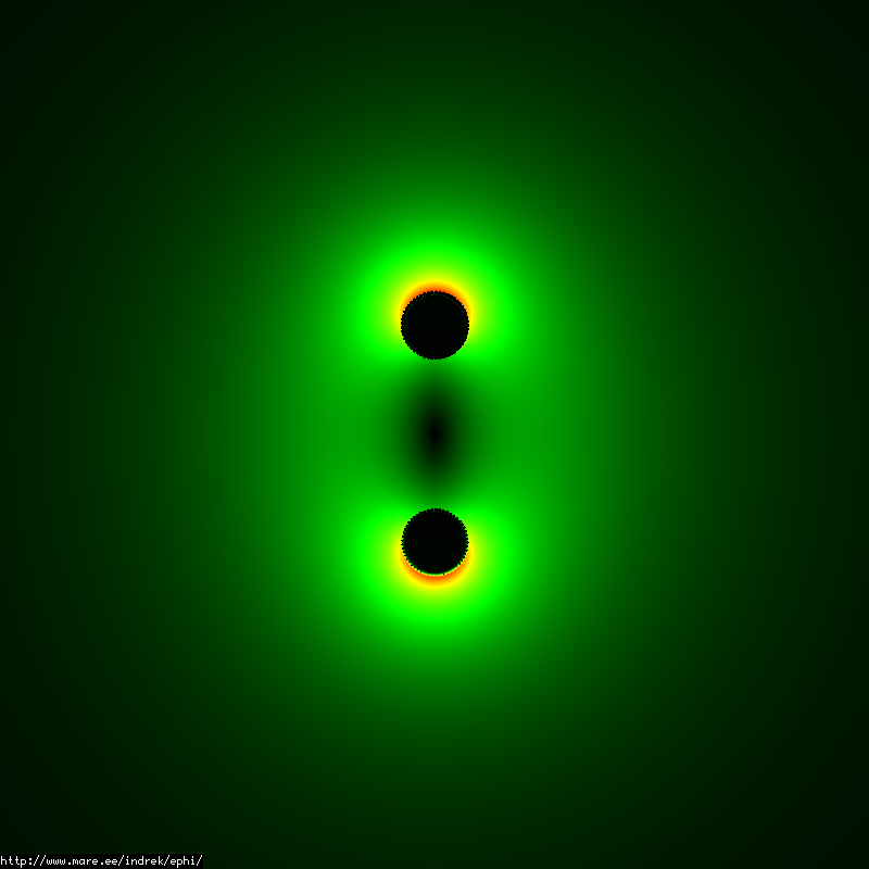
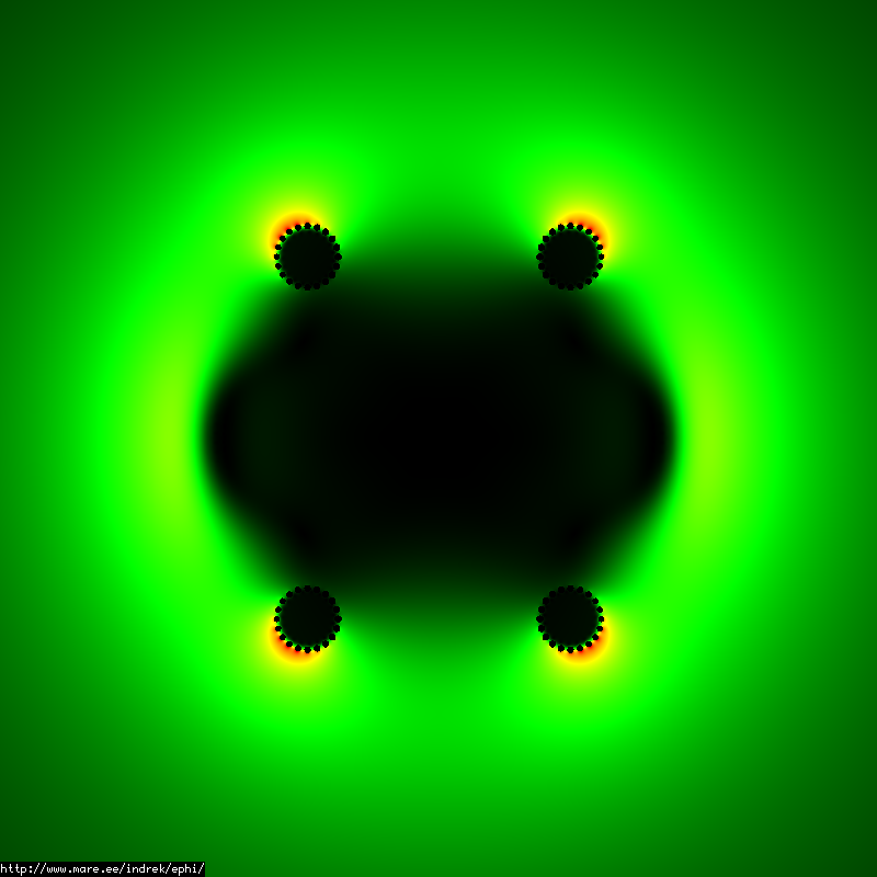
Here's the efield magnitude:
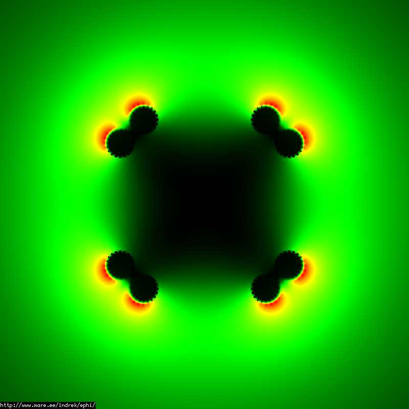
Here's the efield magnitude at logarithmic levels:
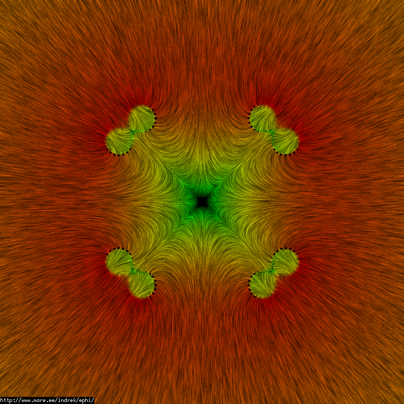
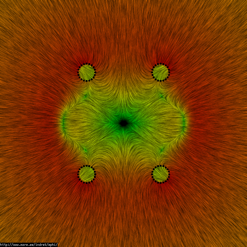
Here's the efield lines with logarithmic coloring:
Here's the efield magnitude:
Here's the efield magnitude at logarithmic levels:
Here's the efield lines with logarithmic coloring:
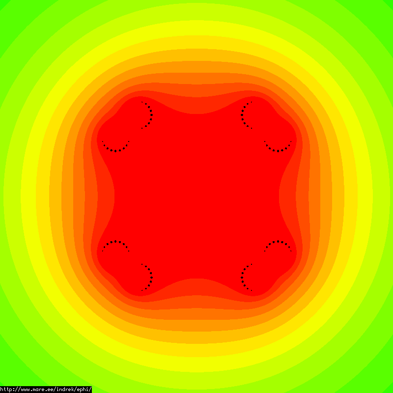
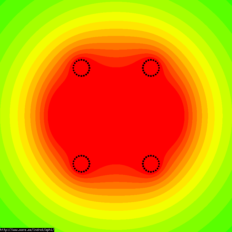
One remaining question: where on the coils is the charge concentrated at? Green indicates less charge, red more charge. I apologize for the bumpy image.
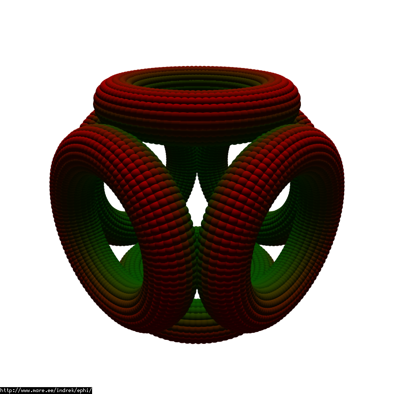
This looks like some poisonous frog. Now what happens if there is a huge negative charge in the middle of the system? Would be interesting to find out. Some other day perhaps.