Lets continue from the previous coil interpolation methods, this time introducing bicubic interpolation. What I found is that compared to the bilinear interpolation the bicubic interpolation is several orders of magnitude more precise at low resolution (<100 MB). With larger (> 500MB) megabyte-against-megabyte grids the distinction is not that great but still in the order of 5-10 times.

In case of the bicubic interpolation it makes sense to calculate the interpolation factors beforehand and store them. So when a value is interpolated we don't have to look up the four grid points but can instead rely on one cell alone. This will reduce the amount of random memory accesses (from 4 different locations - or two times two consequent accesses - to a single access) but the penalty is in memory usage. Also calculation overhead is reduced. Precalculated tables use 4 times more memory. But compared to the bilinear interpolation the bicubic interpolation with precalculated tables takes 16 times more memory for the same grid size. The gain in precision though offsets that handicap.

Another critical element of bicubic interpolation of the coil fields is the precise calculation of the derivatives at each grid point. Any imprecision here will adversely affect the result. This calculation can either be done by numeric differentiation as in my current implementation. It would be better to use analytic forms that are completely within the grasp for coil calculations - one just has to do the mind-numbing work to grind out the equations - as analytic forms for the e- and b-fields are available.

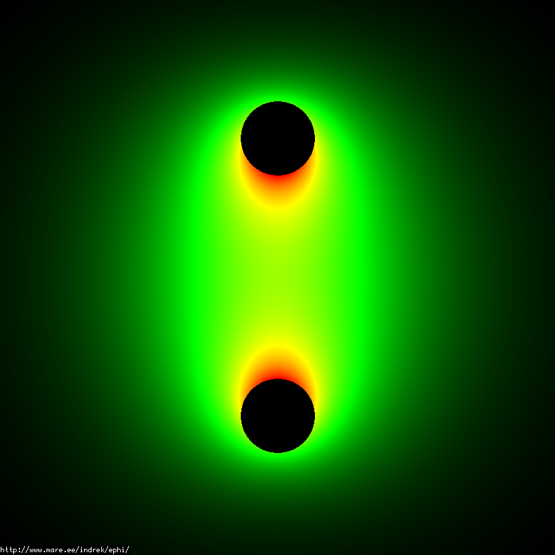
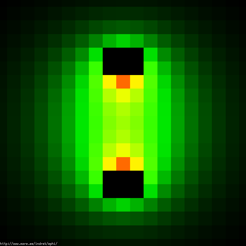
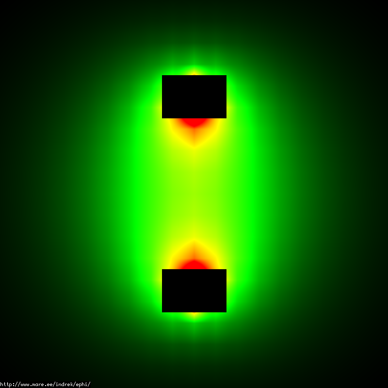
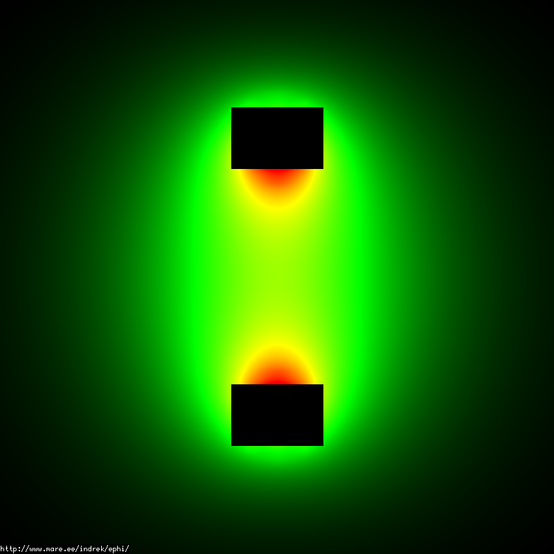
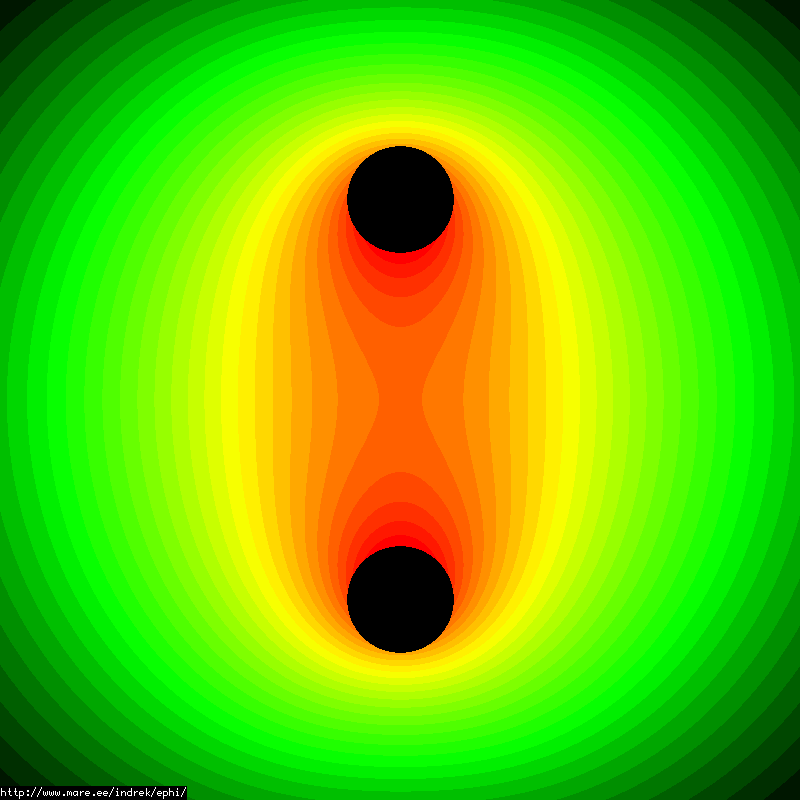
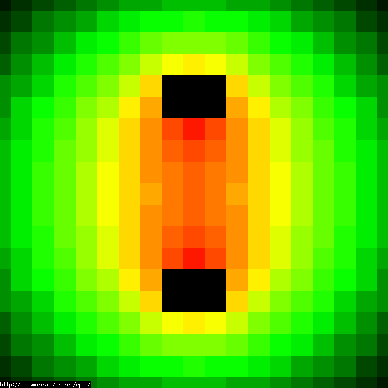
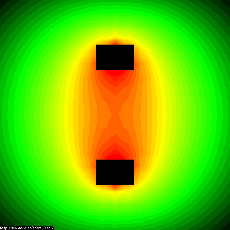
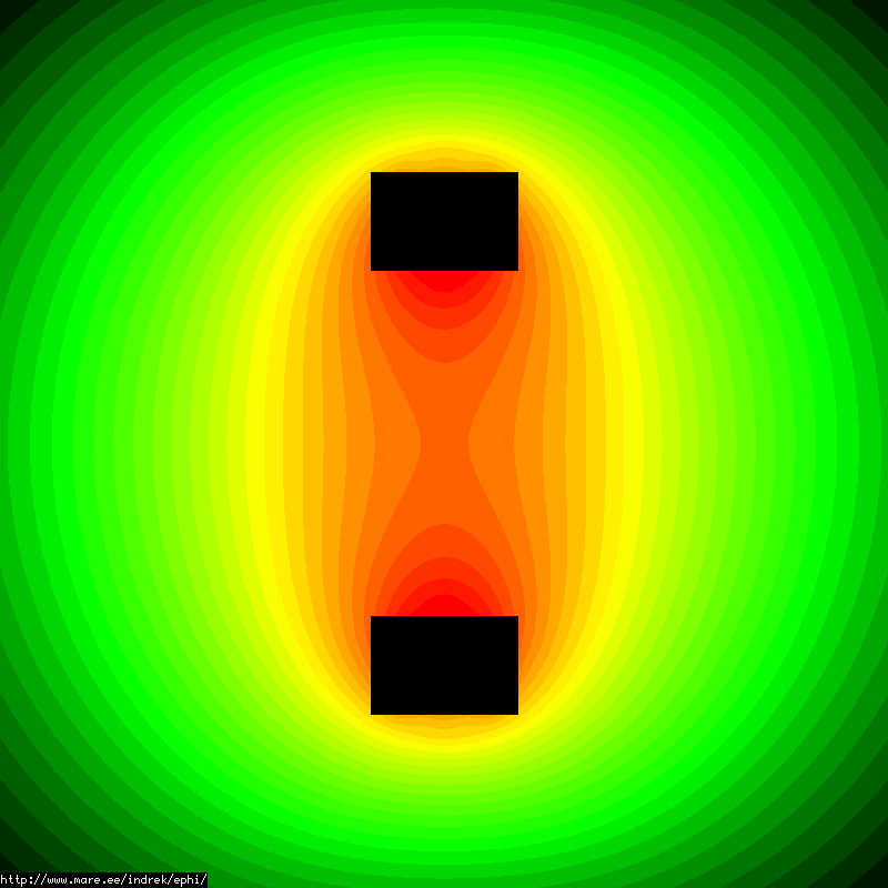
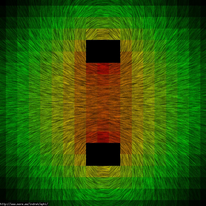
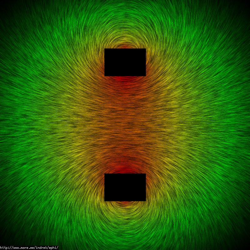
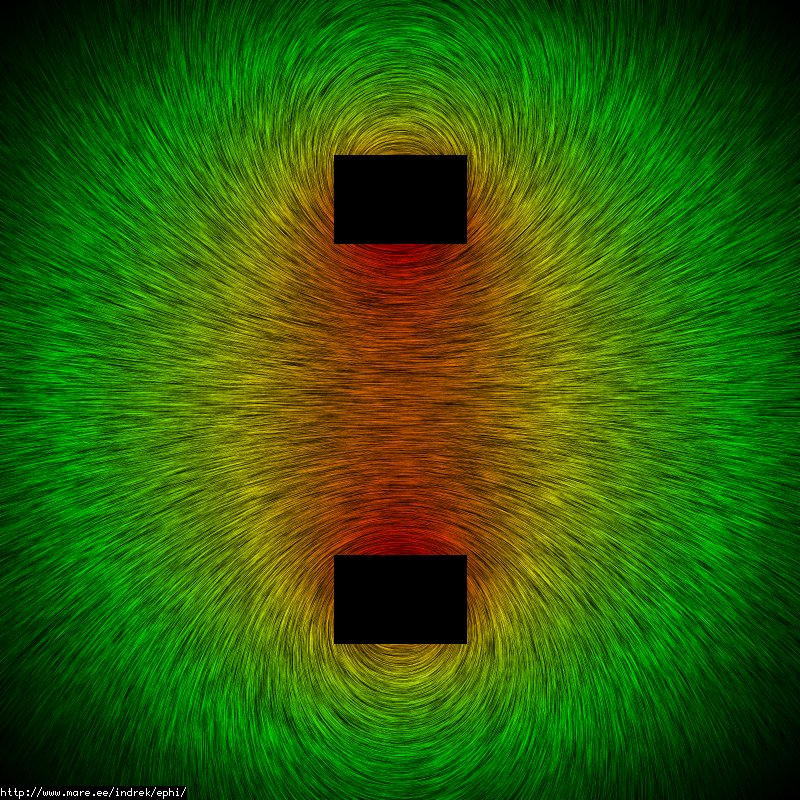
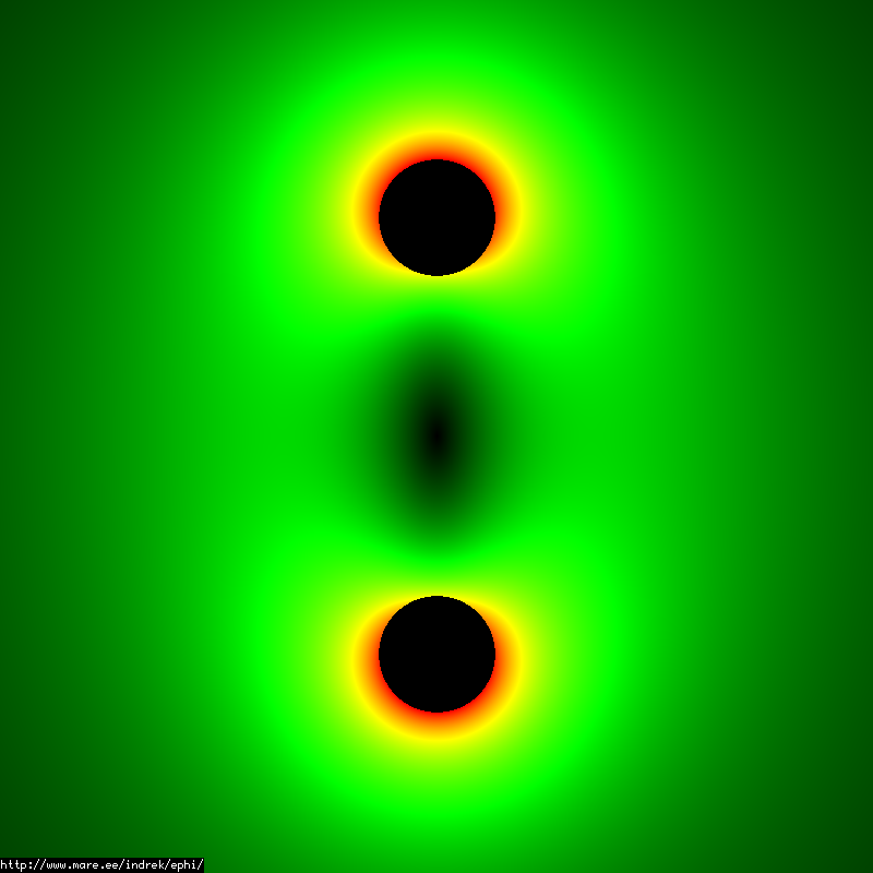
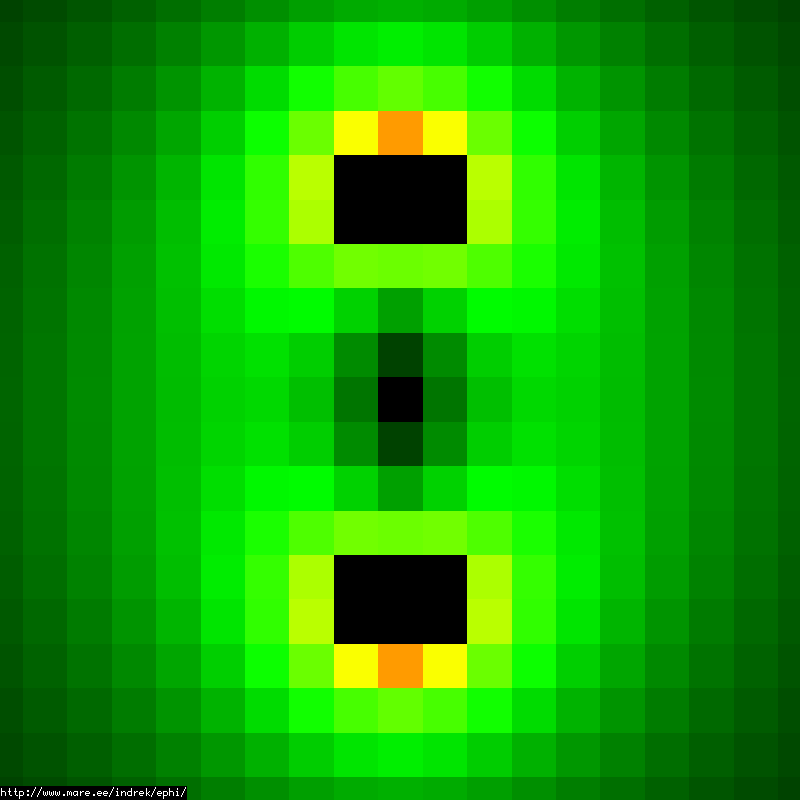
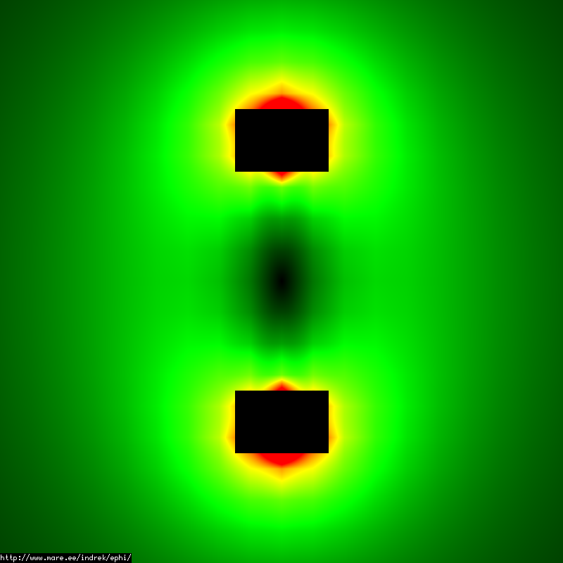
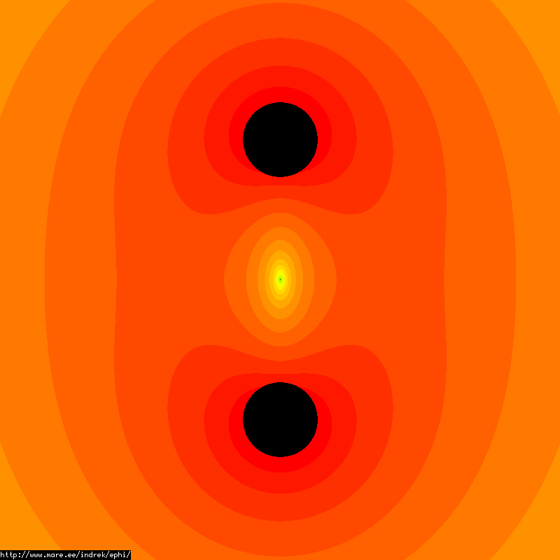
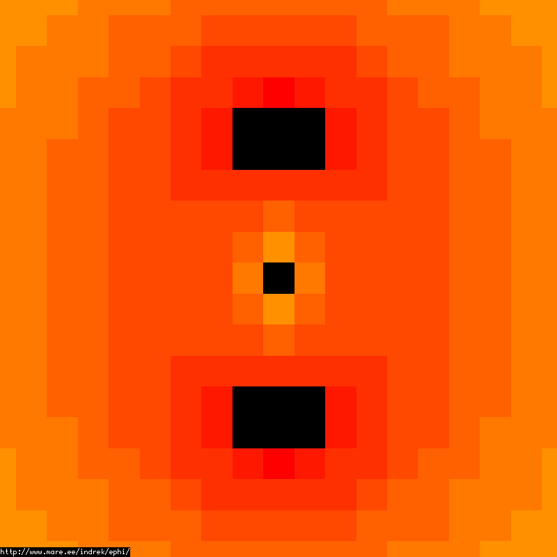
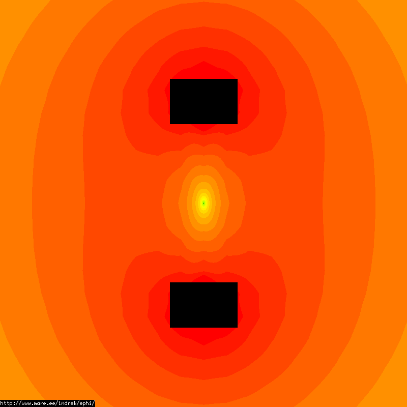
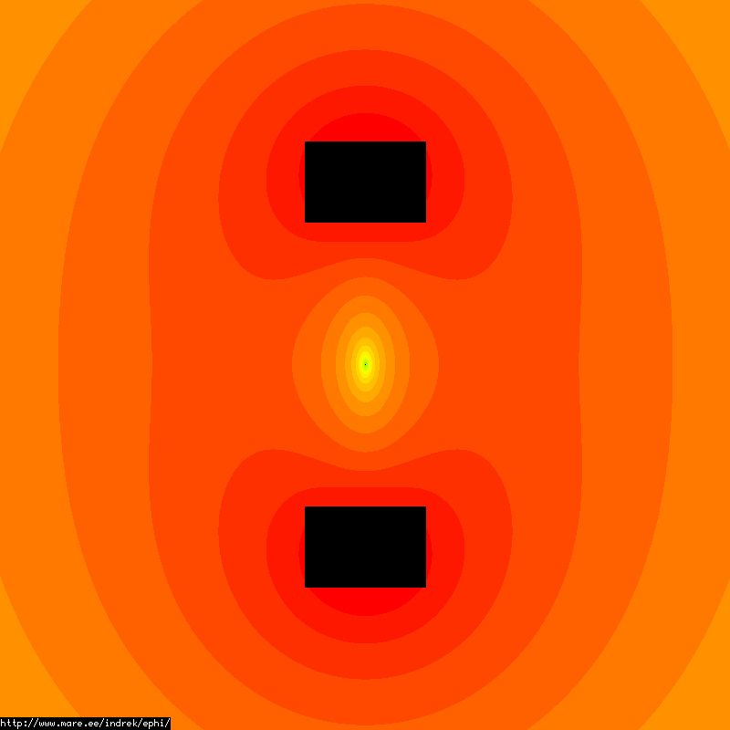
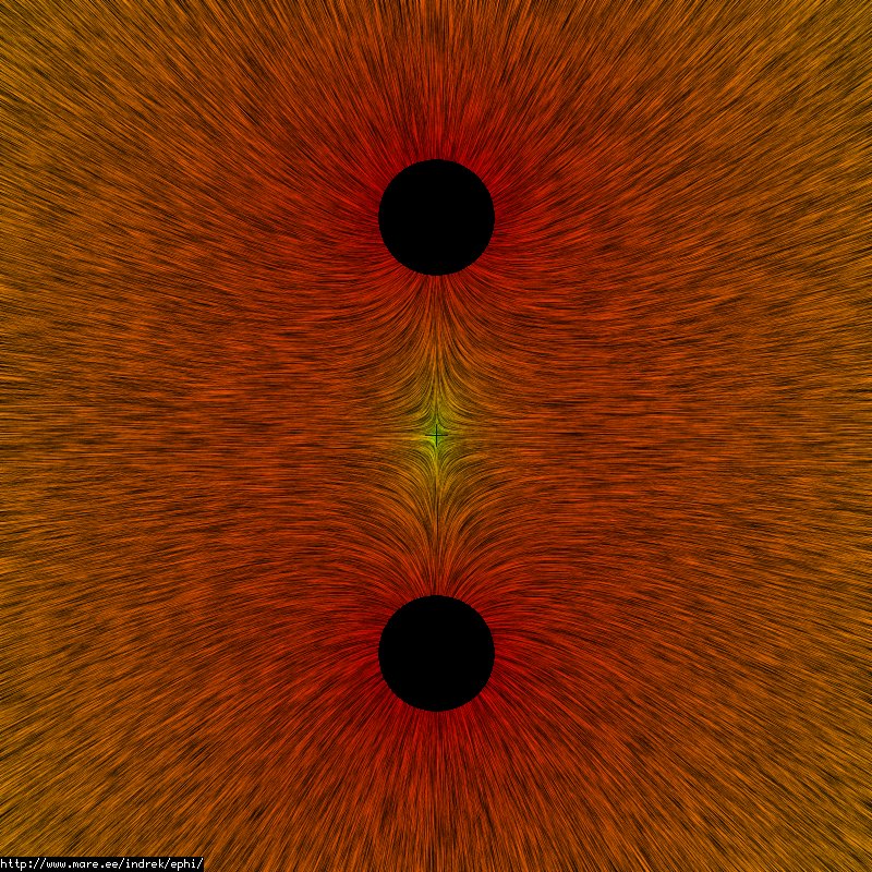
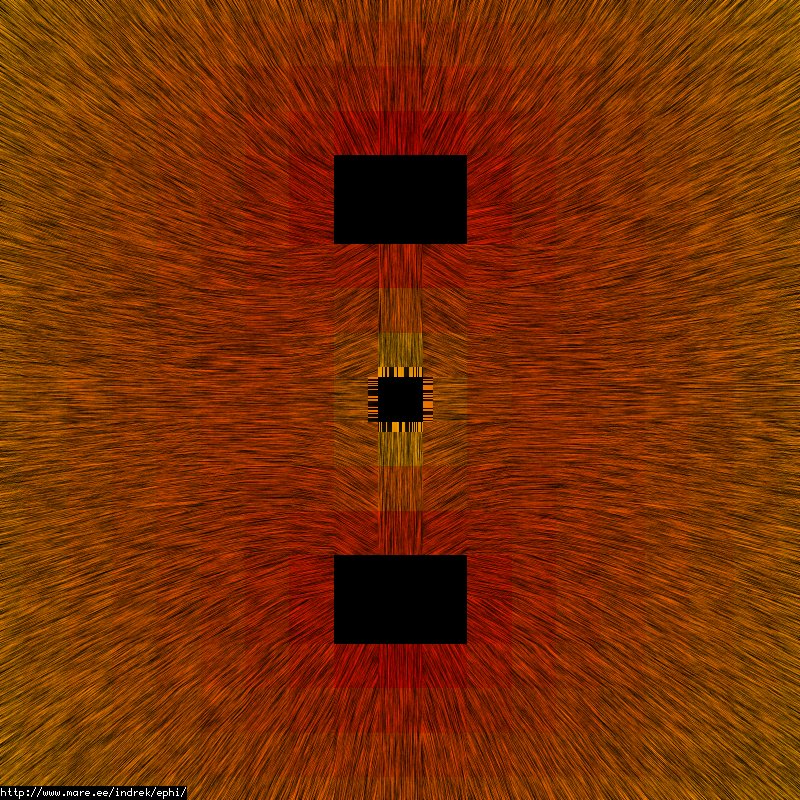
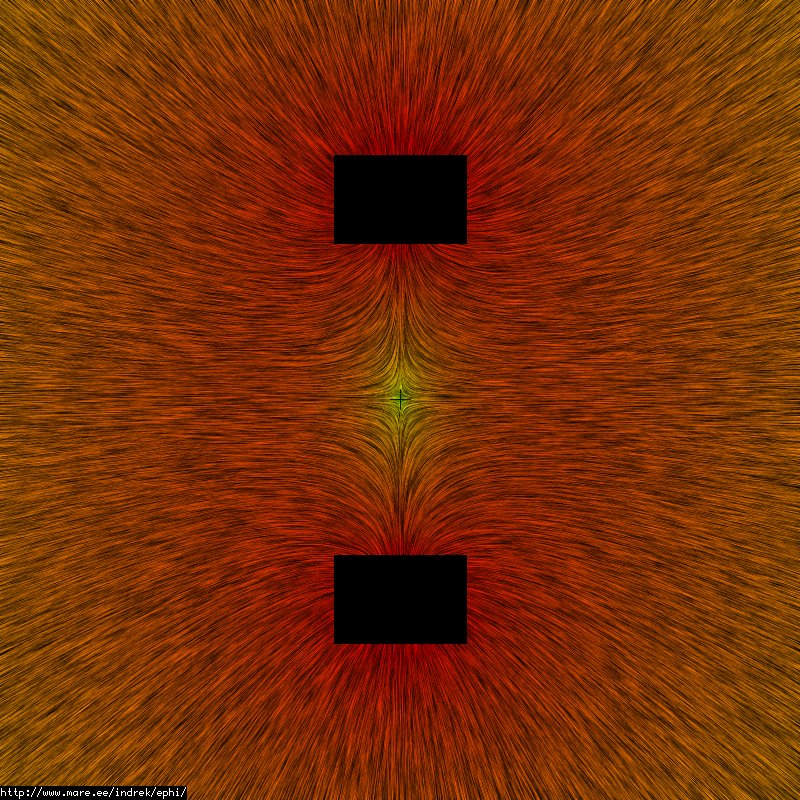
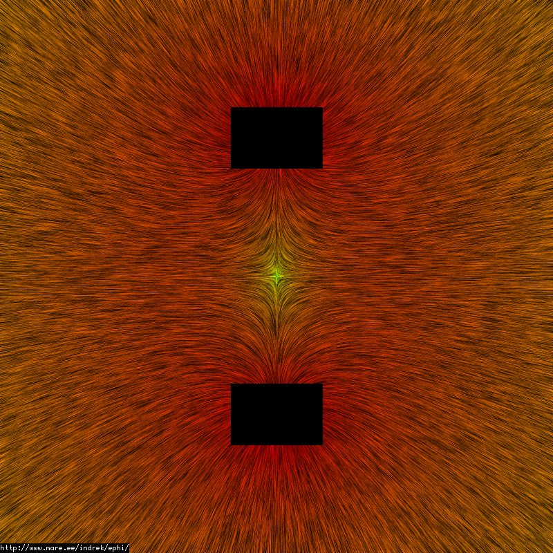
Here you can see the b-field and e-field of a simple circular current (or uniform charge for e-field) element at different interpolation chemes. You can click on pictures to get a better view.