Octave/Matlab B-field calculations for a loop of current and the cube polywell

NOTE: the scripts and info on this page are old and superseded by my dedicated octave page.

Octave is a free programming language and environment for mathematical calculations and data visualization. It closely mimics the commercial Matlab language and functionality.

This is my first Octave code - for calculating the magnetic fields within a cube polywell. The math uses an analytic solution, if you need a reference try chapter 20 from the Dolan's "Fusion Research" book. The formula can also be found from my own ring-of-charge derivation (at the end): efield_ring_of_charge.pdf. The solution uses elliptic integrals though and I've bundled the ellipke.m with the software as the native octave currently seems to lack it. I pinched the code for it off a random website so I'm not entirely certain of its correctness at the moment but it seems to work ok. If you run my code under Matlab you should use the native function instead and delete this one.

Download the code: mbfield-0.1.zip

A few comments about the code:

• The code is vectorized to the best of my ability. But these are my very first octave/matlab scripts so I'm a complete beginner. If you see an obvious optimization opportunity - let me know.
• As the code is optimized for vectorized calculation it might not be fastest for single particle path or for a field line integration.
• Near the axis of a current loop the calculations can become unstable and can provide some low noise on the radial field value (very small/close to zero but still noise).
• This code has no dependence on the ephi codebase - it's stand-alone.
• It has a bundled ellipke.m of somewhat questionable value. It's only for octave - matlab should have it natively. Not sure how matlab handles things but you might have to delete this file to use the (faster and more accurate) matlab function.

Example: how to caculate the magnetic fields from a loop of current. Here we put the loop of current centered at (0, 0, 0) and on the y-z plane, with radius 0.15m and current 1A. We calculate the B-field from two points, the on-axis (0.2, 0, 0) and the off-axis field at (1, 2, 3):

indrek@home:~/mbfield-0.1> octave -q
octave:1> loop_bfield3d([0 0 0], [1 0 0], 0.15, 1, [0.2 0 0; 1 2 3])
ans =

   9.0478e-07   0.0000e+00   0.0000e+00
  -1.0611e-10   5.7977e-11   8.6965e-11

octave:2>

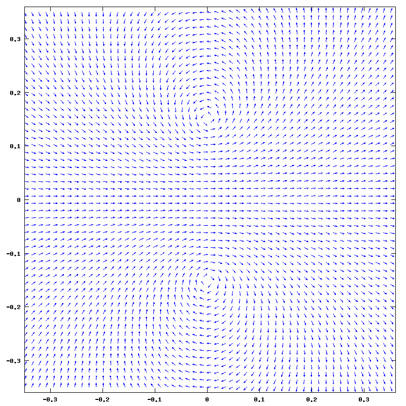
Example: and here's how one would try to visualize the field through a quiver plot.

# get the field sample for the arrows
[x, y] = meshgrid(-0.35:0.0137254901:0.35, -0.35:0.0137254901:0.35);
x = x(:);
y = y(:);
B = loop_bfield3d([0 0 0], [1 0 0], 0.15, 1,
  cat(2, x, y, zeros(size(x, 1), 1)));
# normalize the bfield so we get same sized arrows
B = B ./ repmat(sqrt(dot(B, B, 2)), 1, 3);
Bx = B(:, 1);
By = B(:, 2);

# plot the data with simple arrows
quiver(x, y, Bx, By, 0.016)
print ("loop_arrows.png", "-S800,800"); 

Resulting in an image:

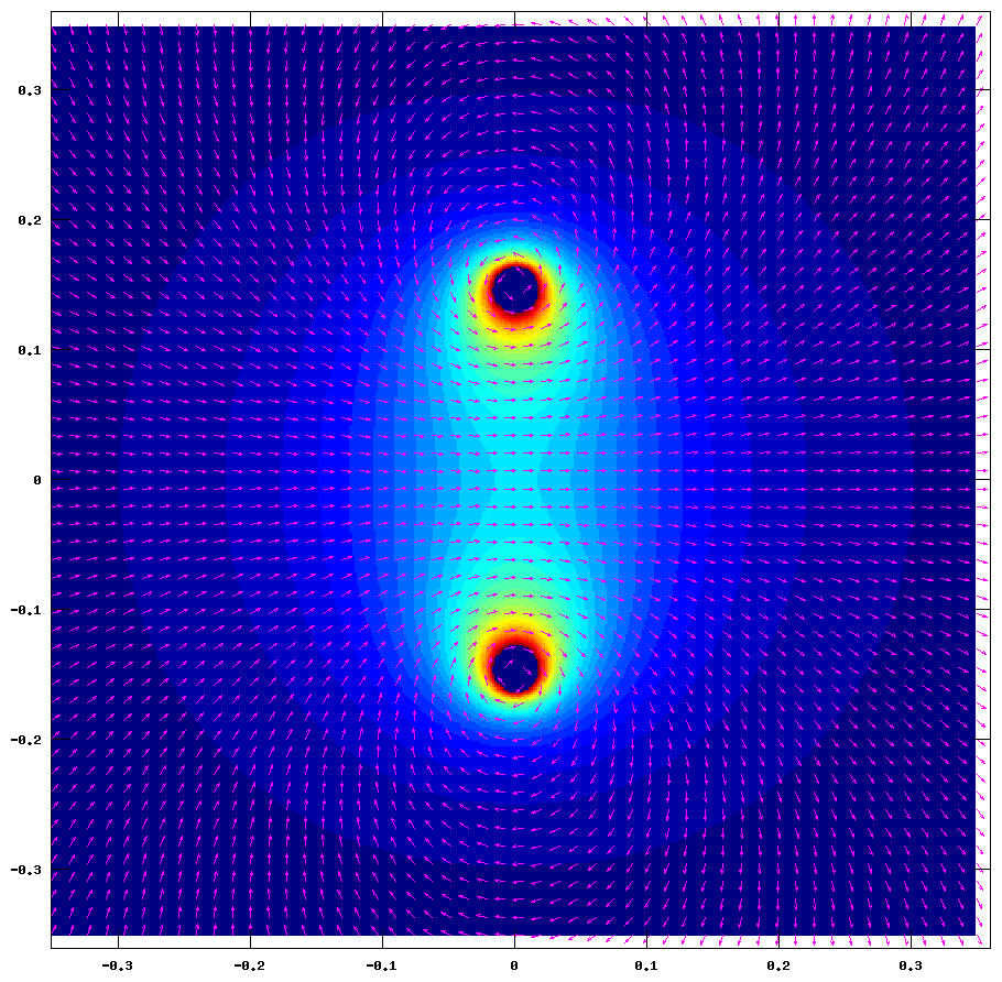
Of course this image lacks field magnitude, so we could do with a bit of color:

# octave does not do pcolor interpolation (at least not for me)
# so we have to get a much thicker sample of field values
[rx, ry] = meshgrid(-0.35:.0018:0.35, -0.35:.0018:0.35);
B = loop_bfield3d([0 0 0], [1 0 0], 0.15, 1,
  cat(2, rx(:), ry(:), zeros(size(rx(:), 1), 1)));
lv = sqrt(dot(B, B, 2));
rlv = zeros(size(rx));
rlv(:) = lv(:);
# zero the extreamly high field values to get a decent plot
maxbf = norm(polywell_bfield(0.15, 0.08, 1, [-0.25 0 0])) * 5
rlv(find(rlv > maxbf)) = 0;

# get the field sample for the arrows
[x, y] = meshgrid(-0.35:0.0137254901:0.35, -0.35:0.0137254901:0.35);
x = x(:);
y = y(:);
B = loop_bfield3d([0 0 0], [1 0 0], 0.15, 1,
  cat(2, x, y, zeros(size(x, 1), 1)));
# normalize the bfield so we get same sized arrows
B = B ./ repmat(sqrt(dot(B, B, 2)), 1, 3);
Bx = B(:, 1);
By = B(:, 2);

# plot the data with colored background
clf
hold on
pcolor(rx, ry, rlv);
colormap(jet(32));
shading interp
quiver(x, y, Bx, By, 0.016, "m");
hold off
print ("loop_colored.png", "-S1200,1200");

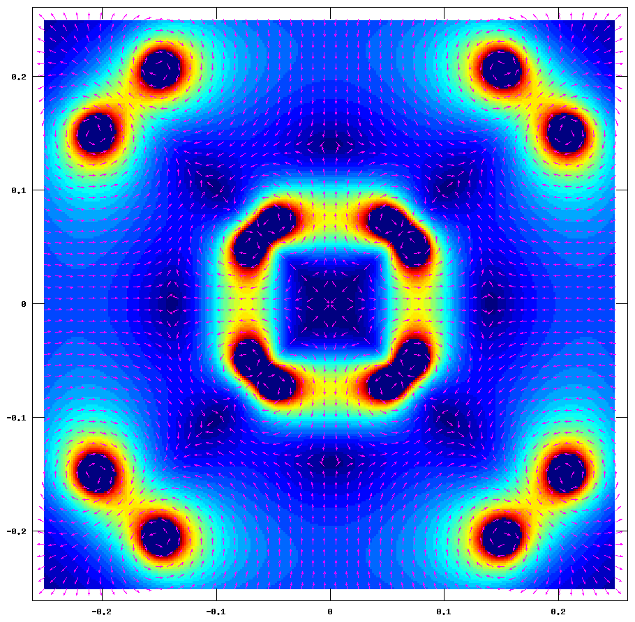
Here's the loop_colored.png:

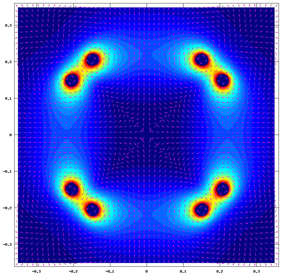
Here's the cube polywell:

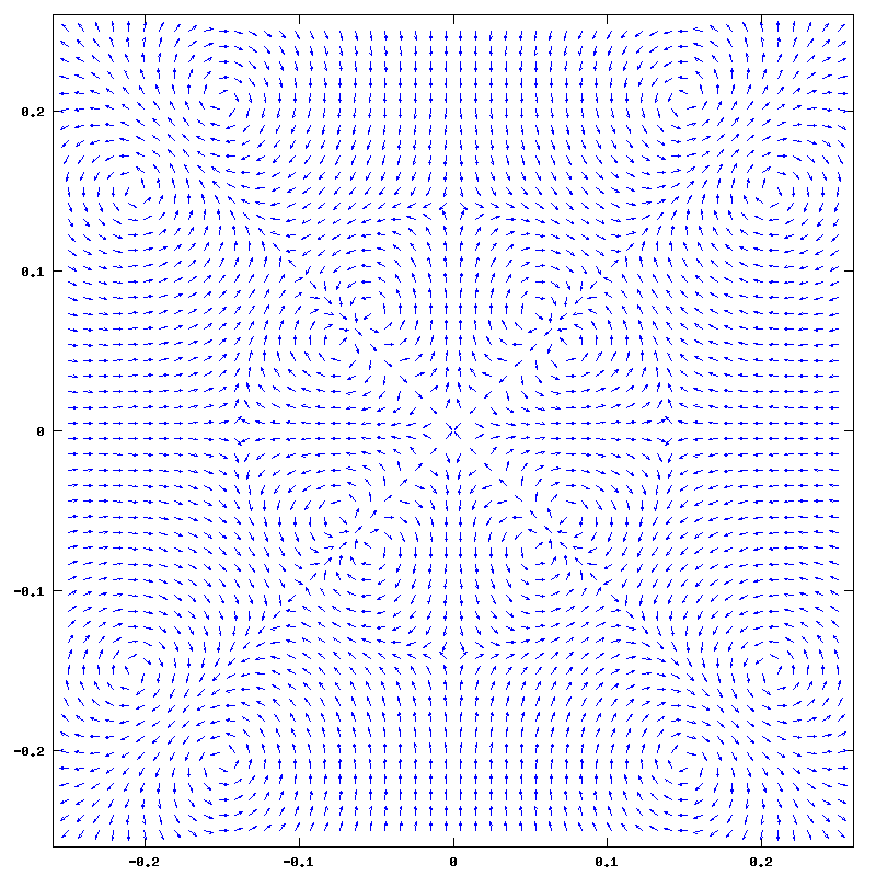
The latest word at wiffleball research seems to be opposed image coils in the middle. Here are a few images on that effect:

Return to ephi..

Copyright © 2008 Indrek Mandre