In our last experiments I let charges literally flow between points on the surface of the conductor. What I realised is that I can write out a series of linear equations on the potential in the conductor against the point charges on the surface of the conductor, solve them, and get an accurate solution.
So we have N points on the surface, each having individual charge q we want to find. We pick another N potential points inside the conductor - where potential is preset and known. What I found what works best is to pick the potential points slightly into the conductor away from the surface and direct vicinity of the charge points.
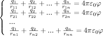
So we have N charge points, N potential points and we get N linear equations. This can be computationally solved using the Gauss-Jordan elimination technique. Lets see how it works.
We start with a sphere again. A 0.25 meter radius sphere set at 1000 volts.
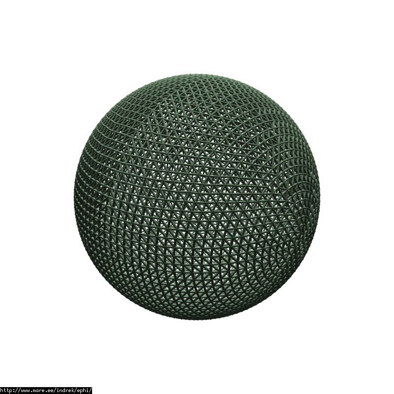
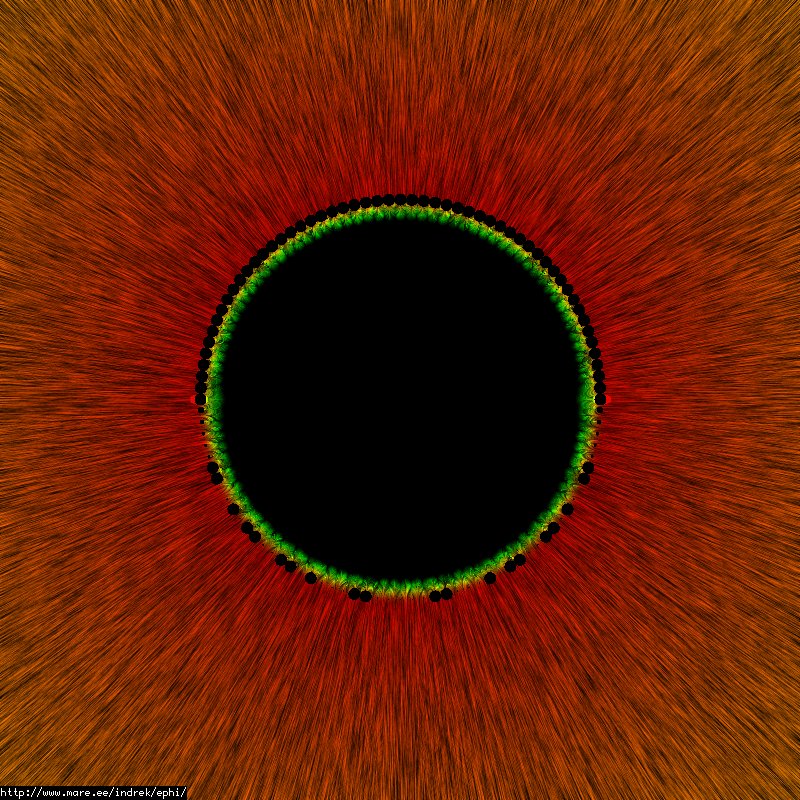
With 3631 points the simulator estimates the capacitance of the sphere as 27.81625140108pF. The theoretical estimate is 27.81625140134pF. Woohoo! Great result. What's more, the field within the sphere really is close to zero, even with logarithmic field view:
Lets try a torus, with major diameter of 0.75m and minor diameter of 0.15m.
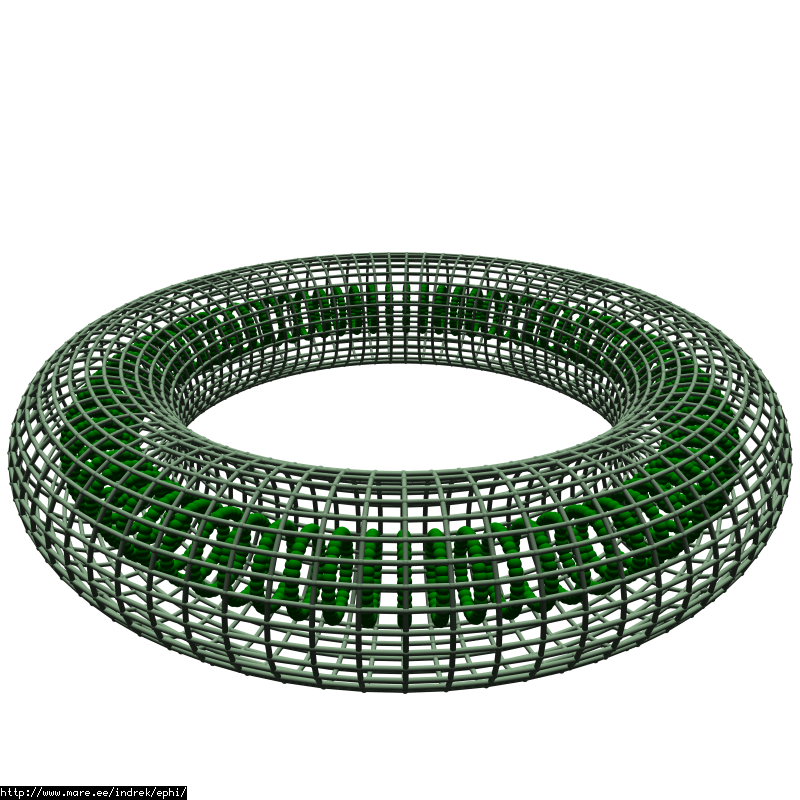
The green dots within are the potential points used. The calculated capacitance is 31.107025888718pF. The value from the http://www.coe.ufrj.br/~acmq/tesla/capcalc.pdf gives us 31.107pF. The numbers match as much as is available. After experimenting with the position of the potential points I've come to realisation that their position and alignment in reference to the charge points is critical. "Good" results only come out when the potential points are directly behind the charge points. I guess this is some special case and not a general solution to arbitrary conductor shapes. One possibility also is that my linear equation solving code is not stable enough or that the linear system only has a good solution if such a symmetry condition is met. Sad :( Still if this method works for toruses then we can build a polywell. Lets just do that and see what happens.
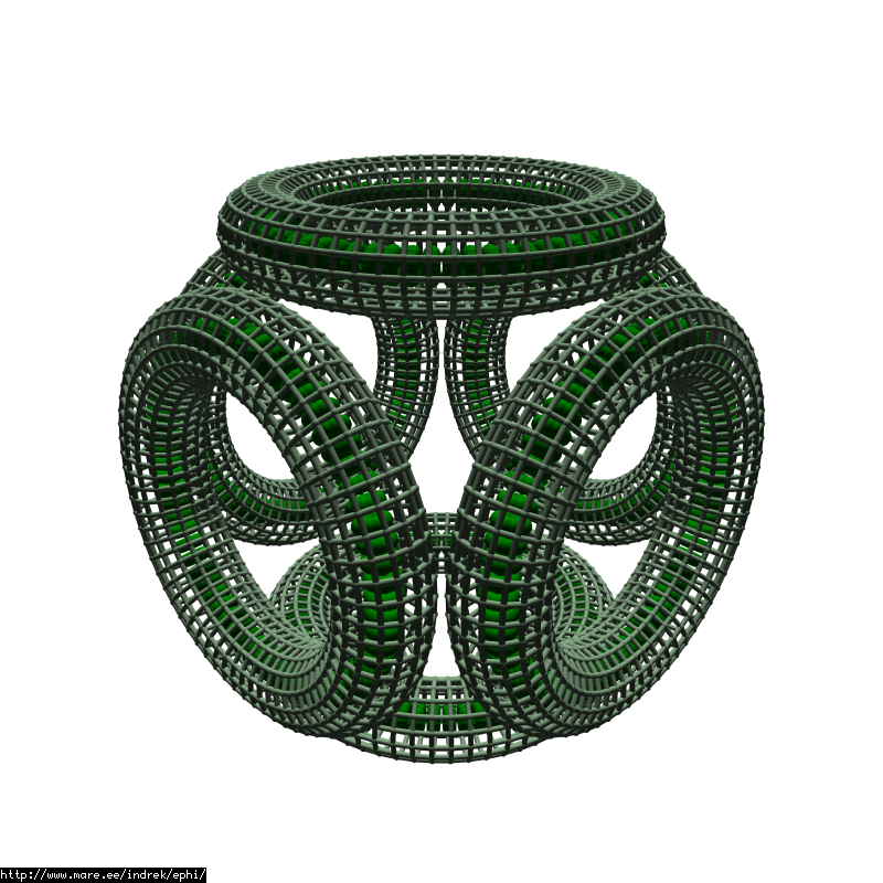
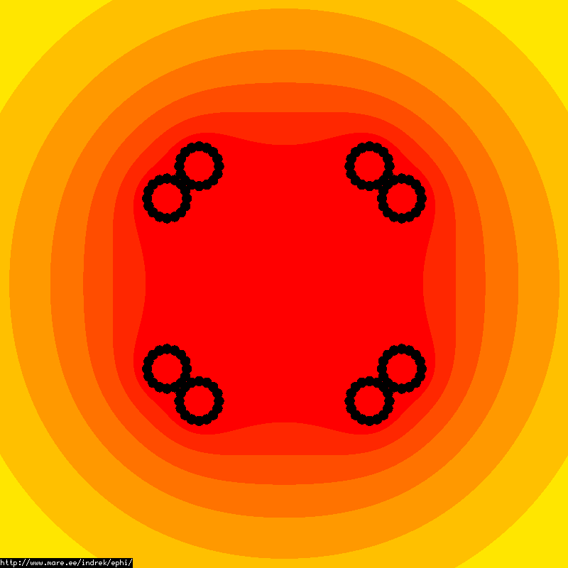
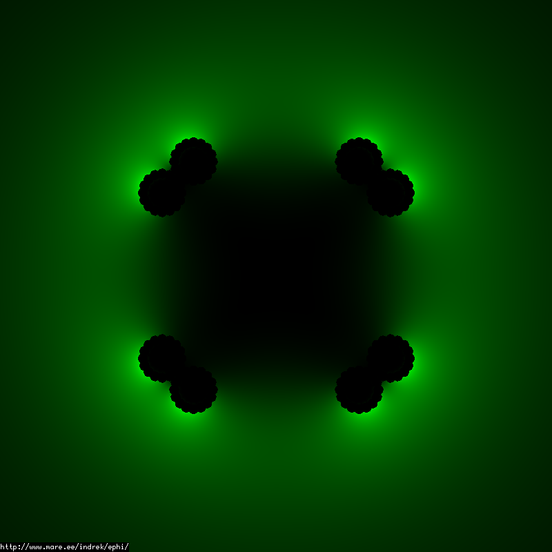
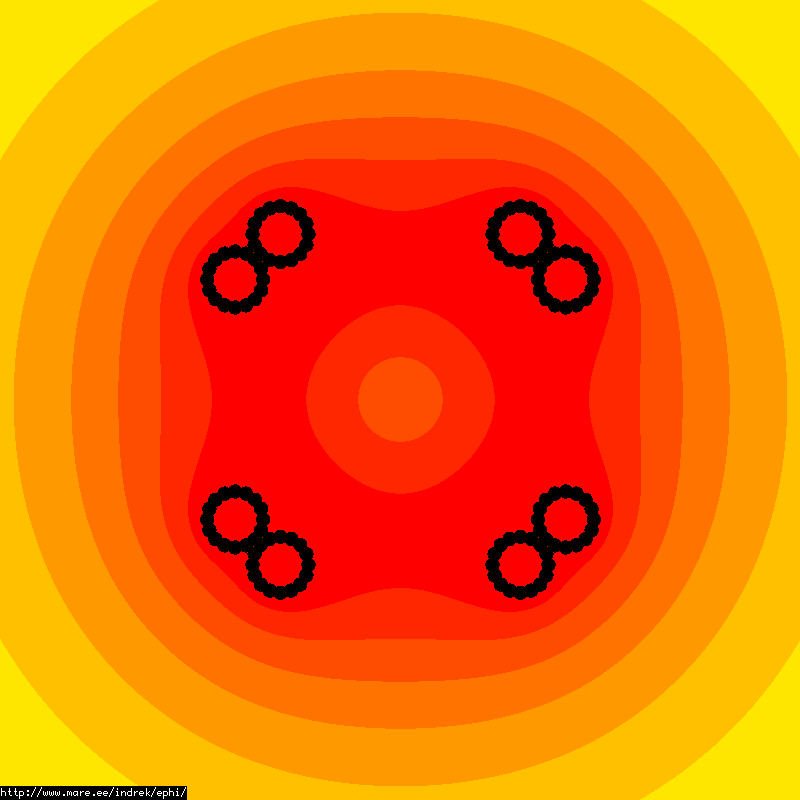
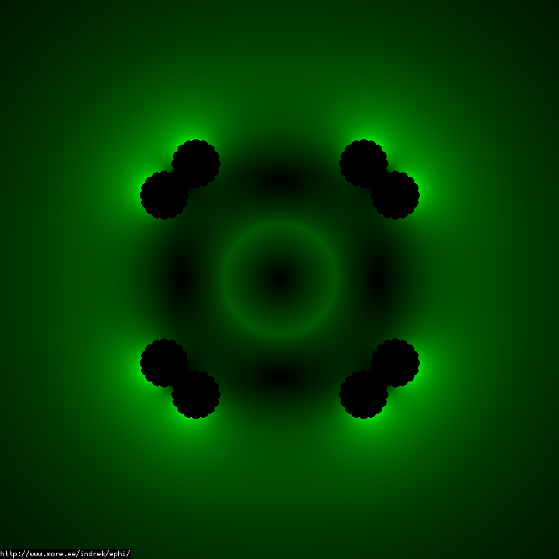
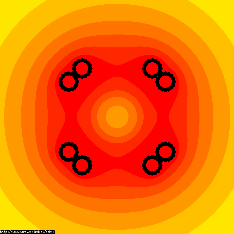
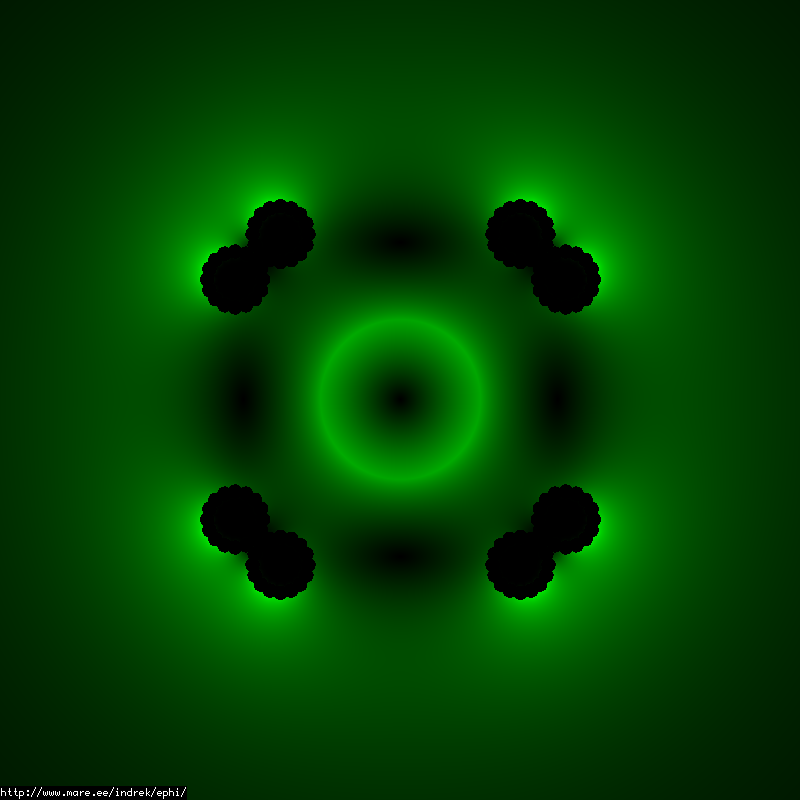
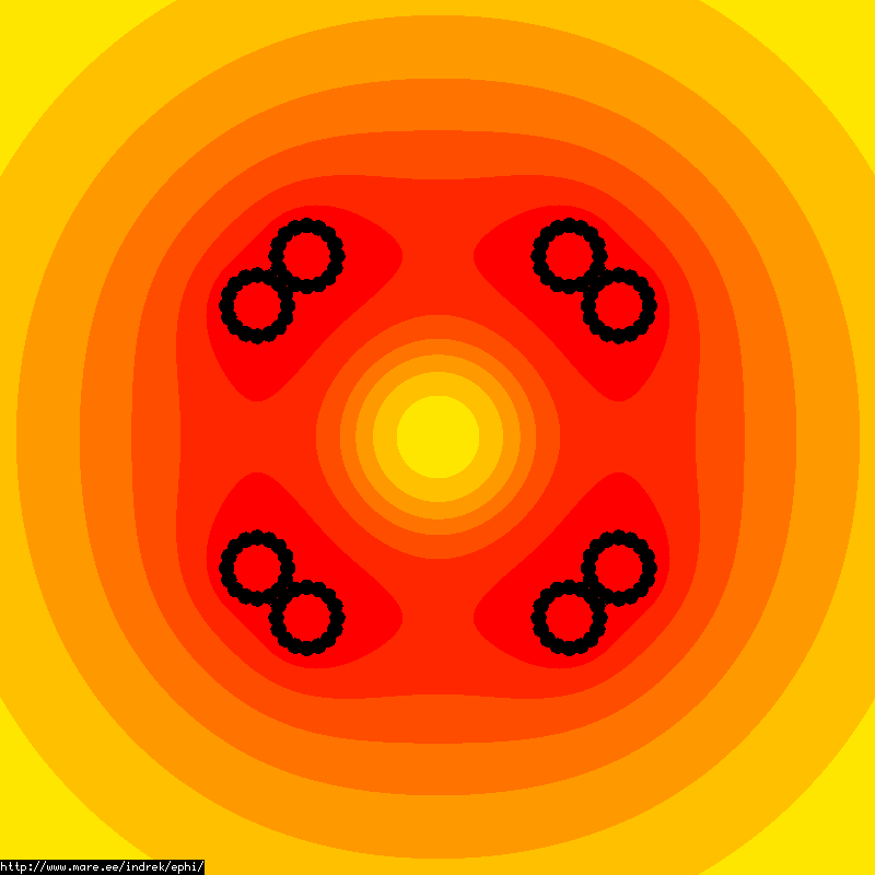
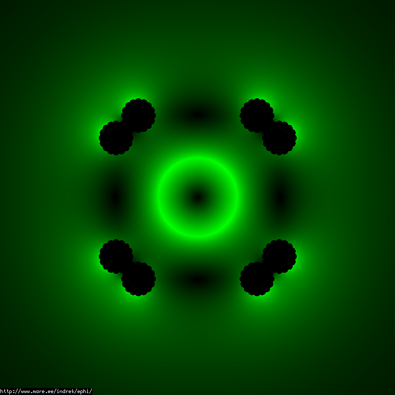
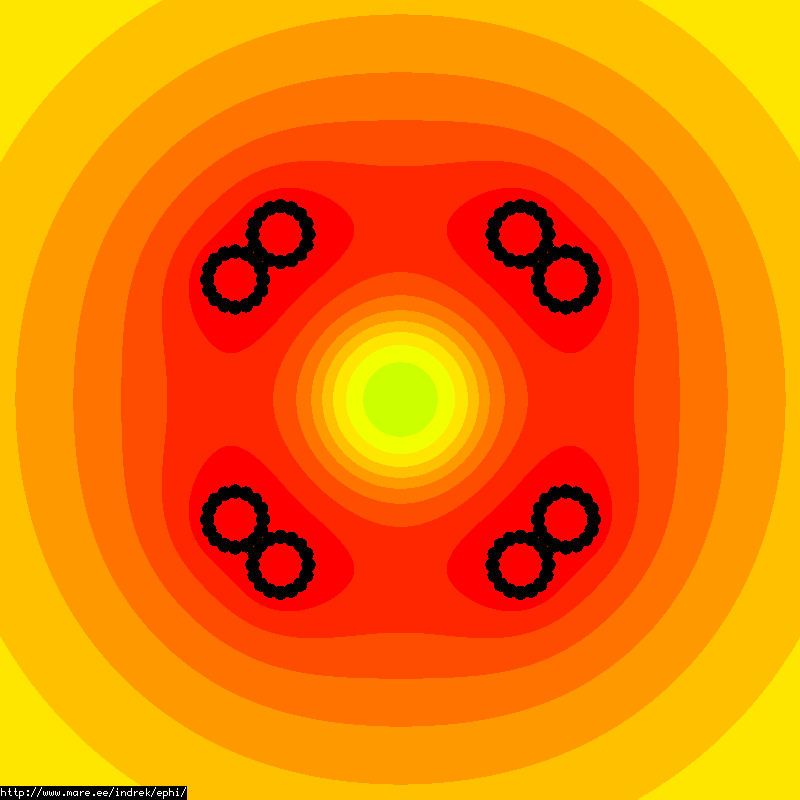
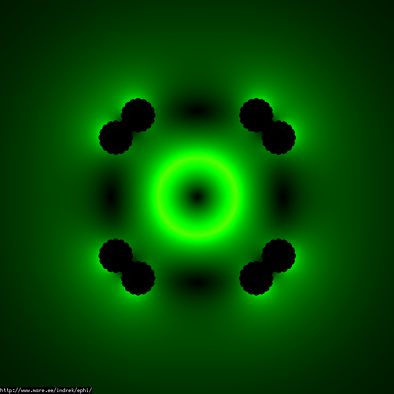
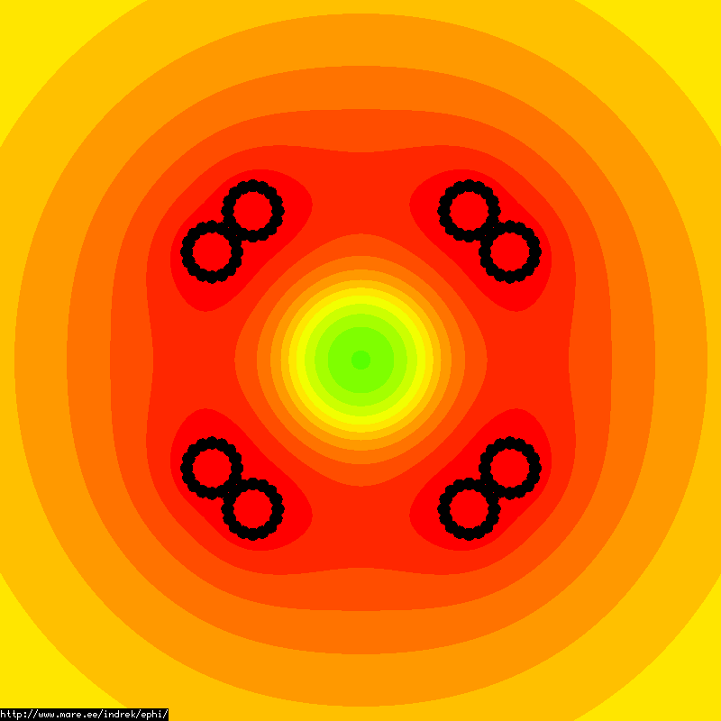
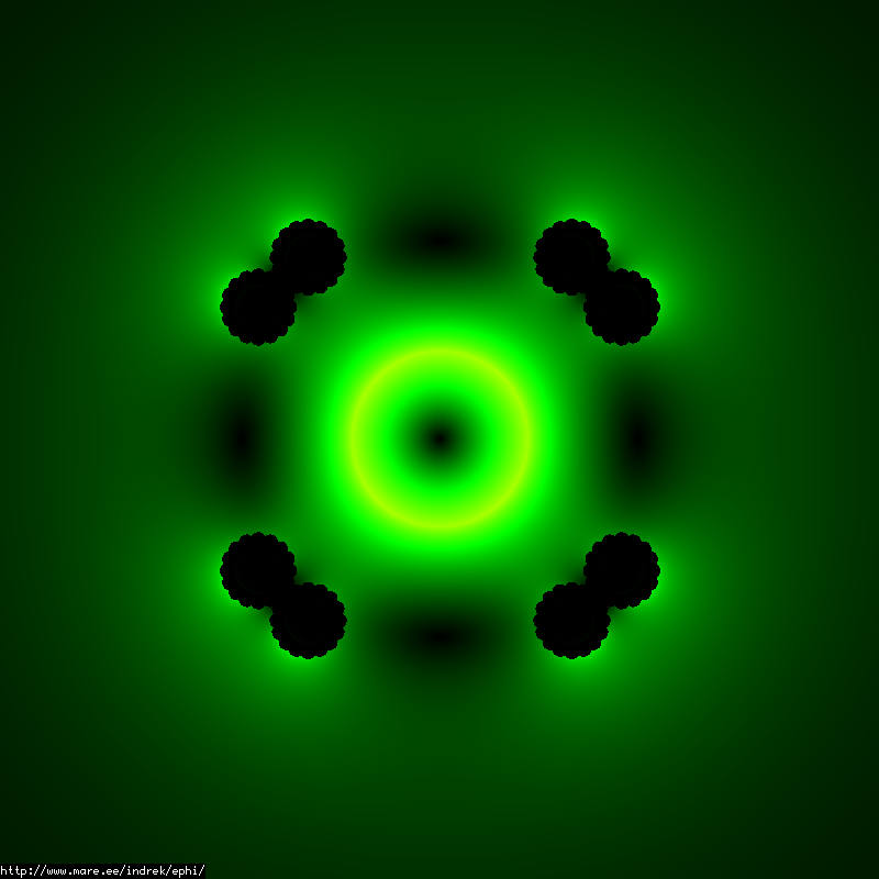
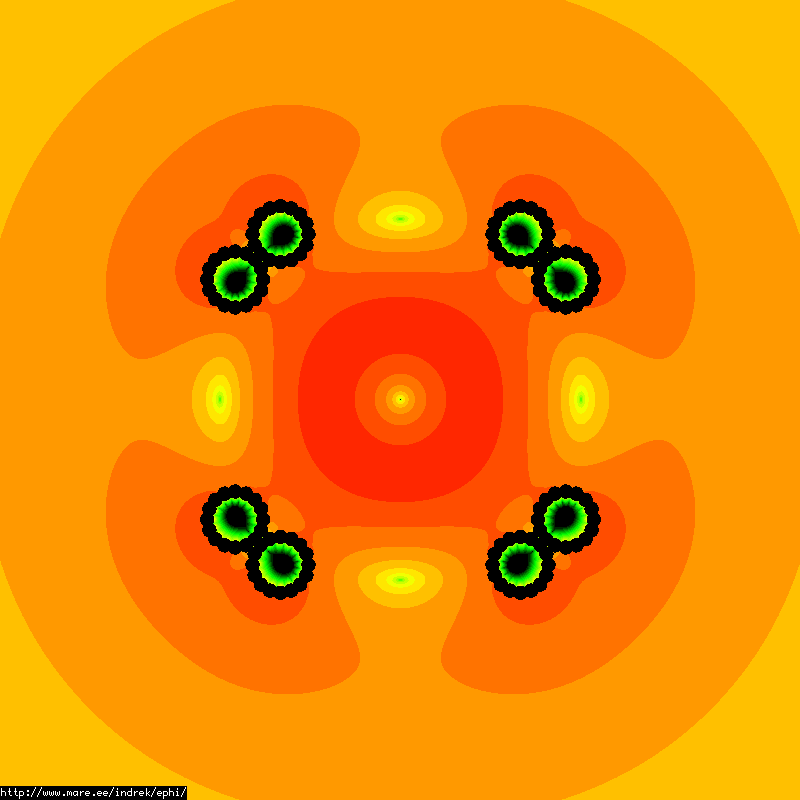
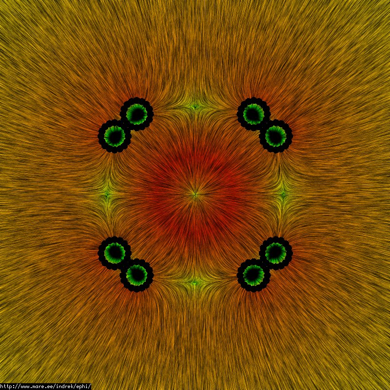
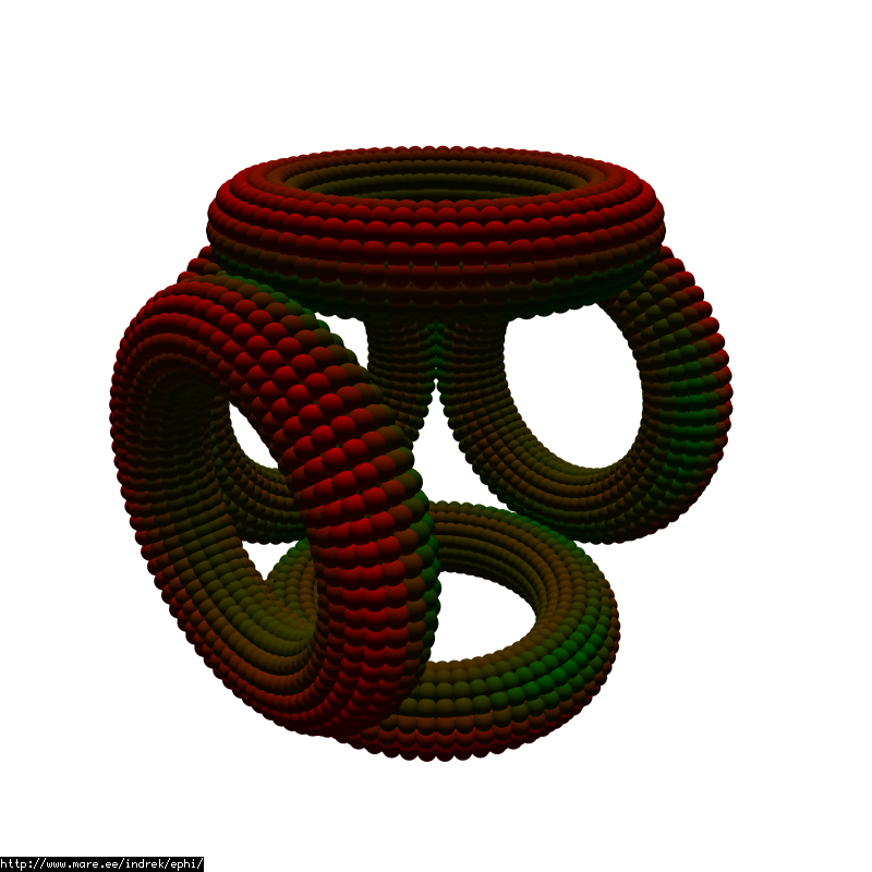
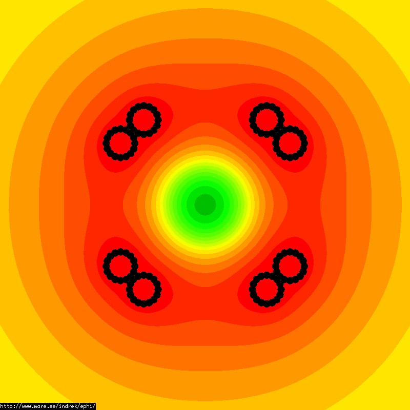
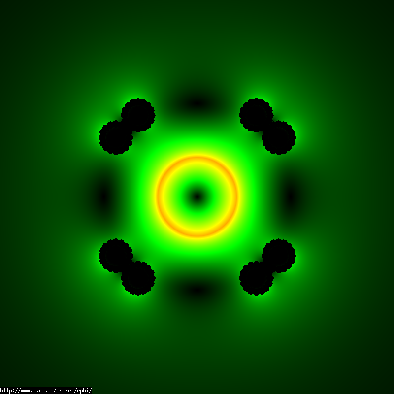
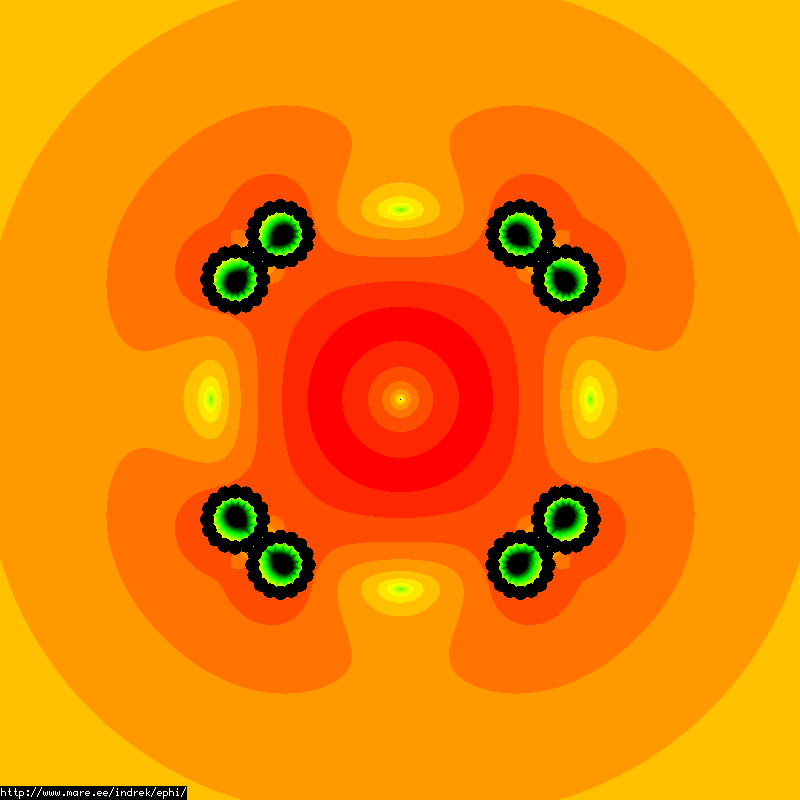
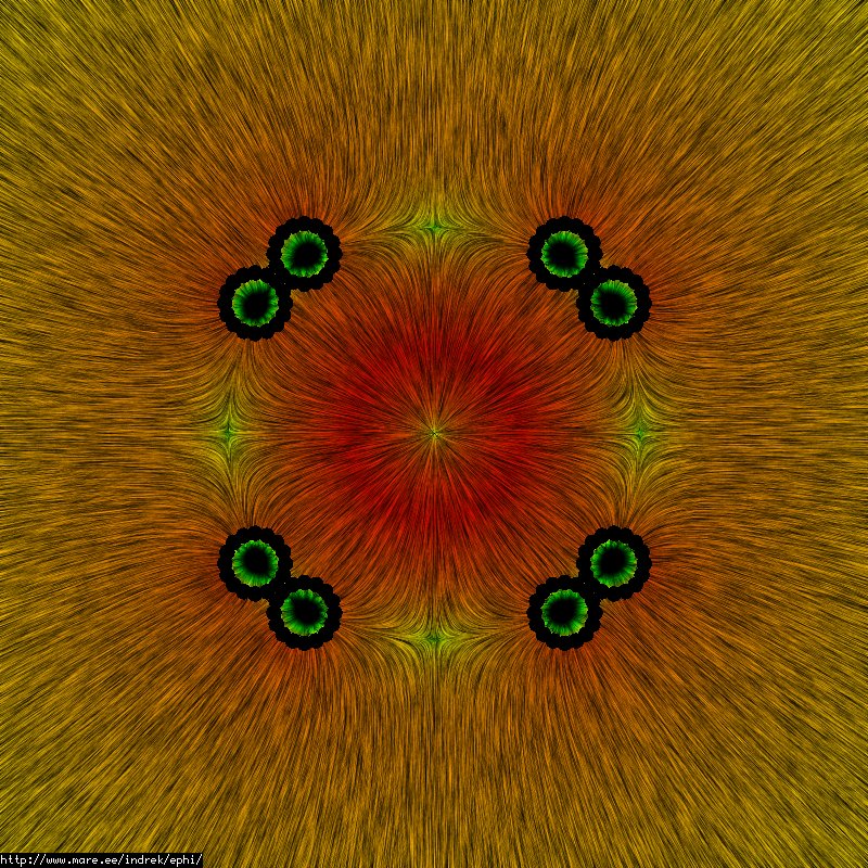
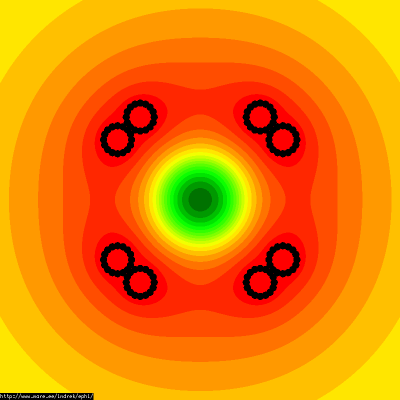
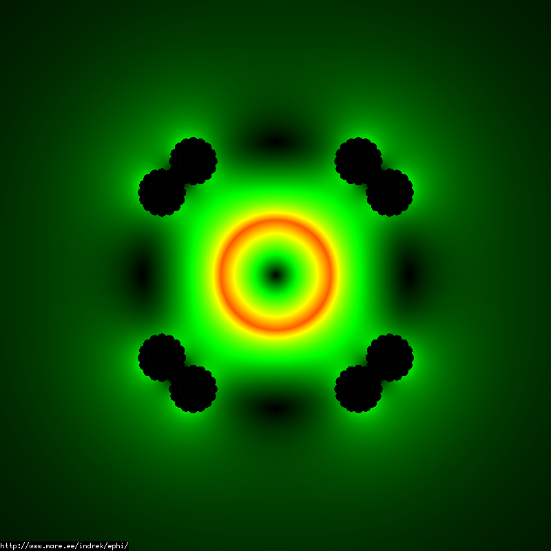
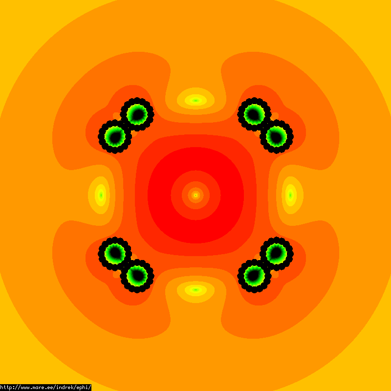
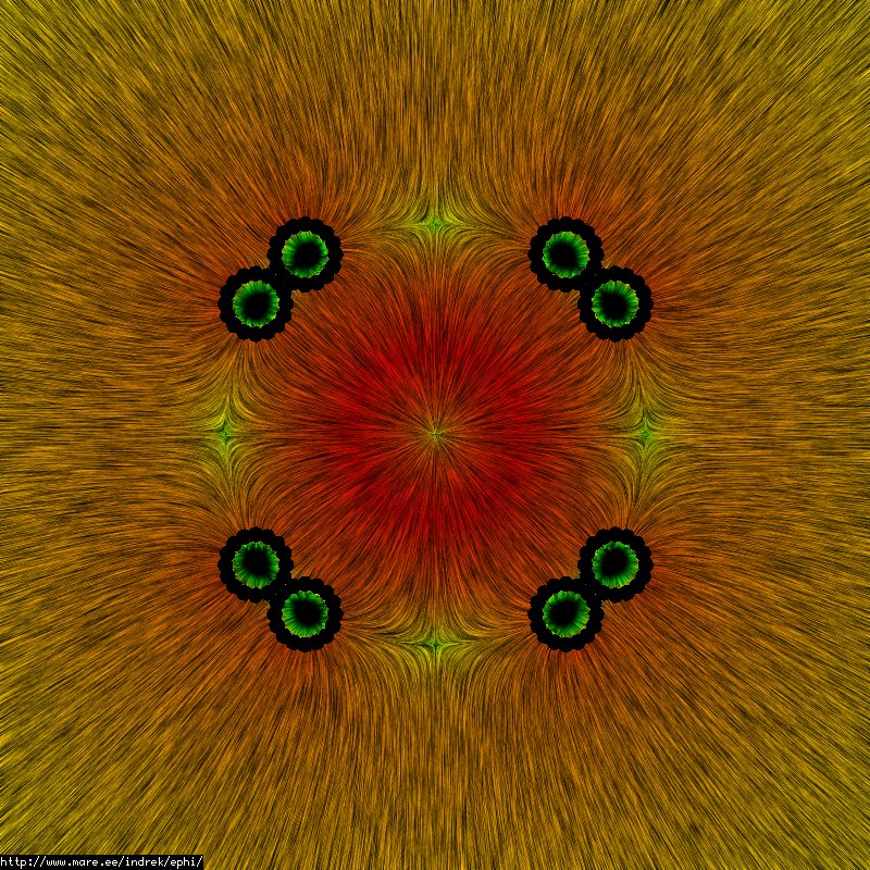
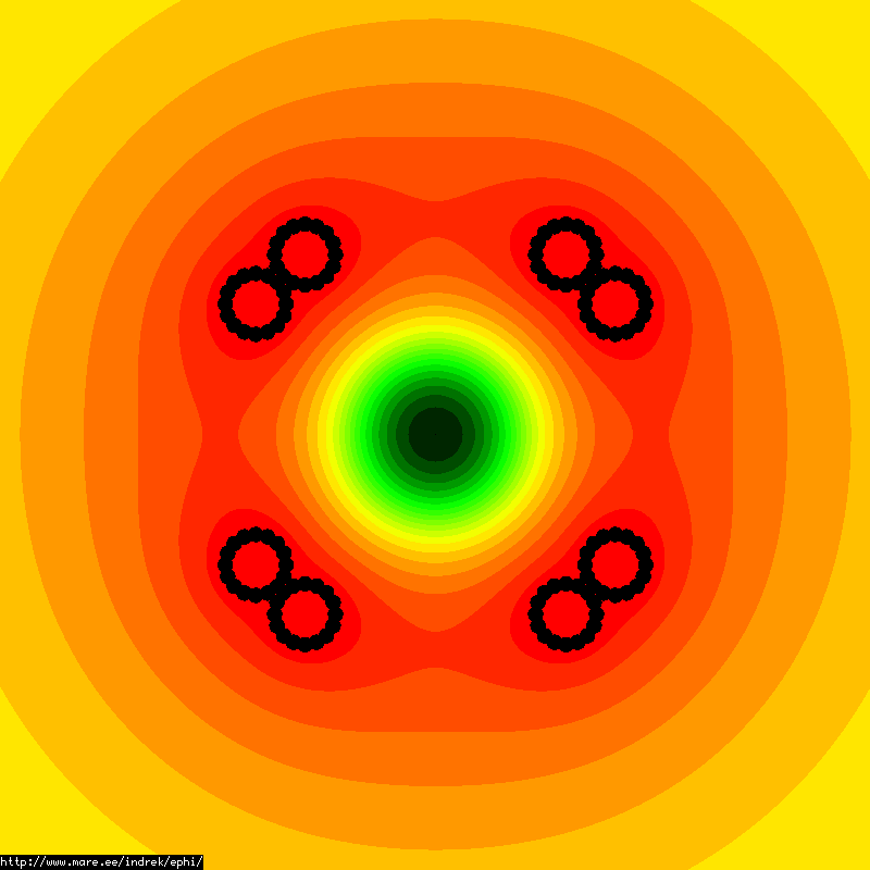
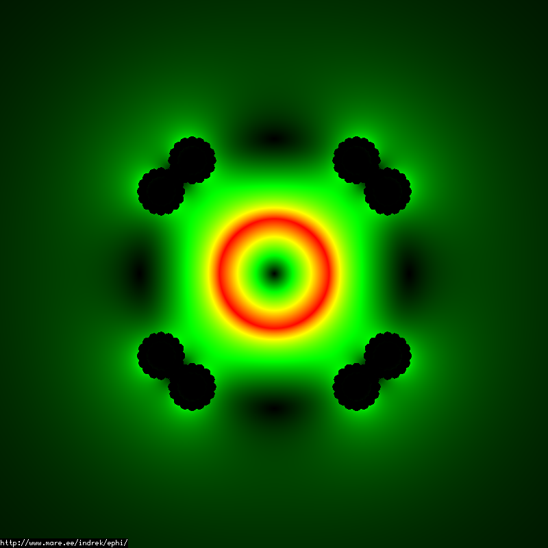
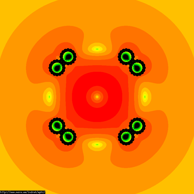
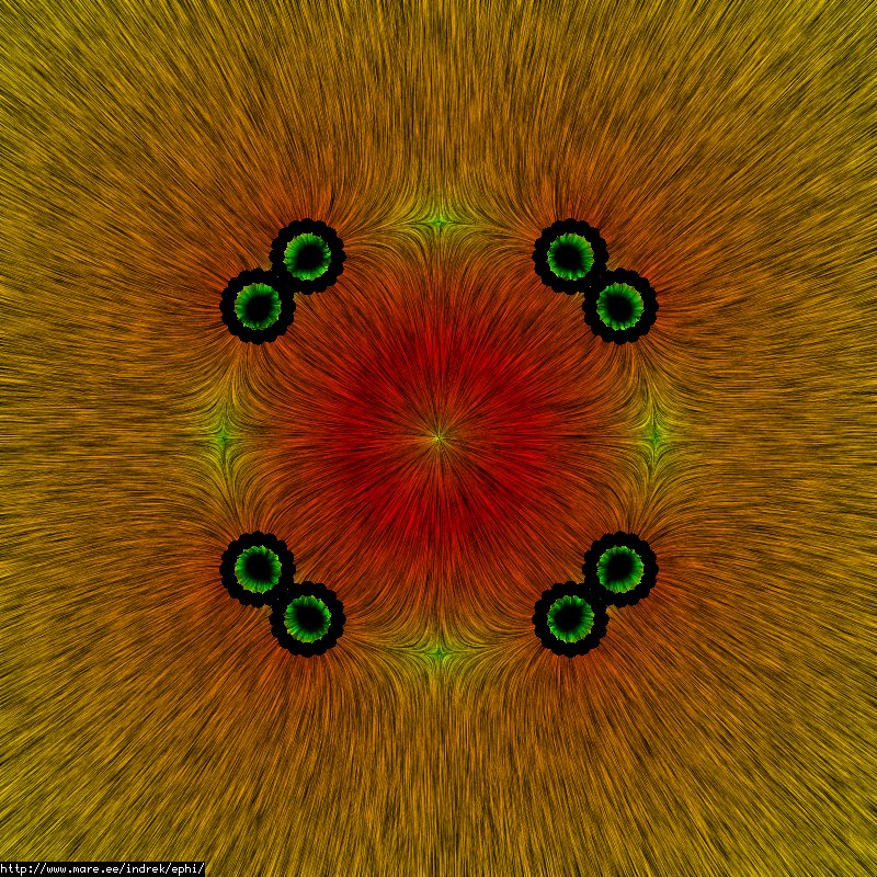
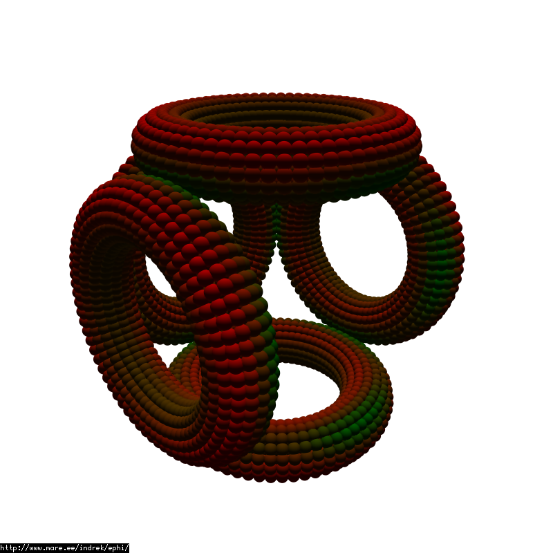
This polywell consists of 6528 points. Radius=0.15m, coil thickness=0.07m, spacing between coils=0.01m. The calculated self-capacitance is 30.1782pF. All the numbers and pictures look correct. Here are the efield lines with logarithmic coloring for the field magnitude:
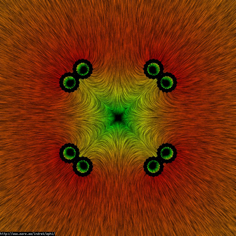
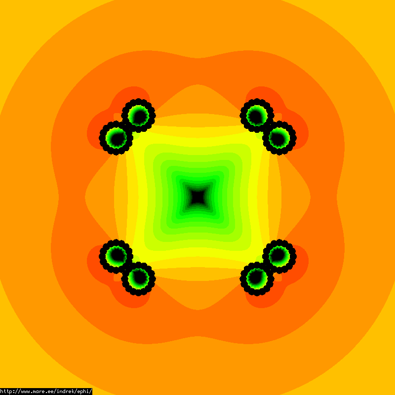
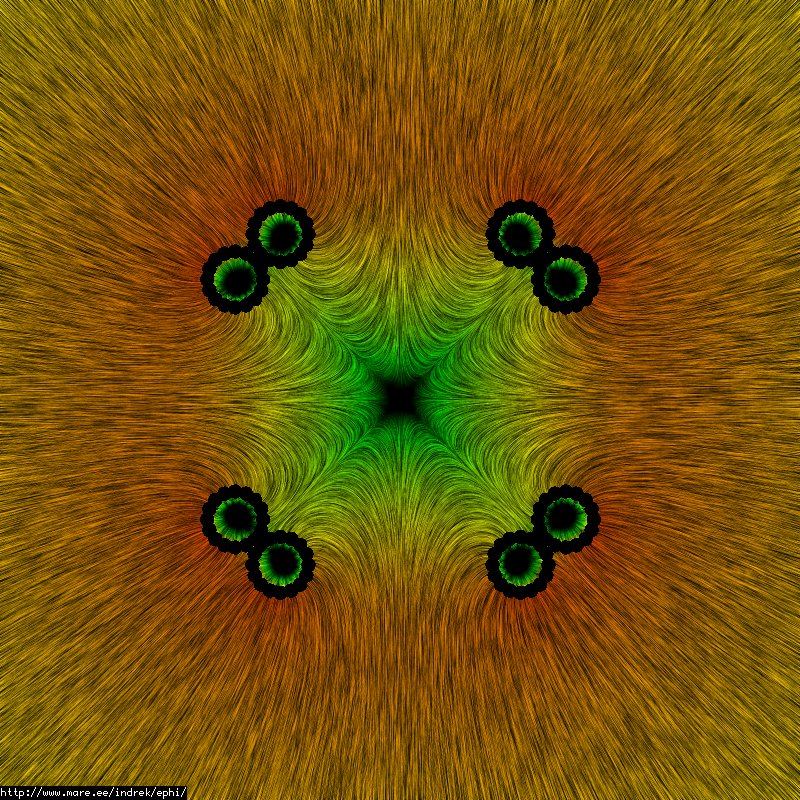
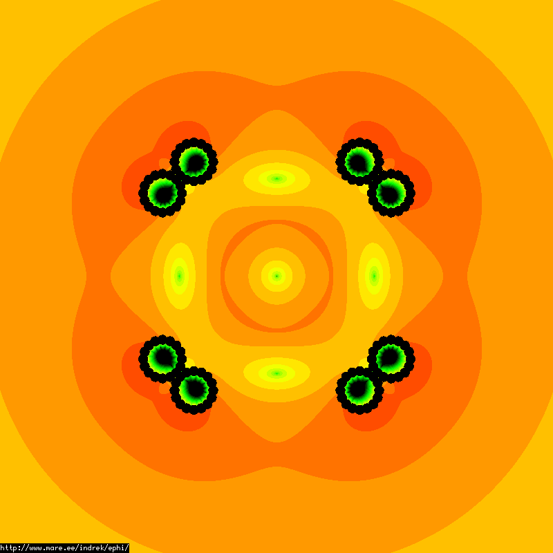
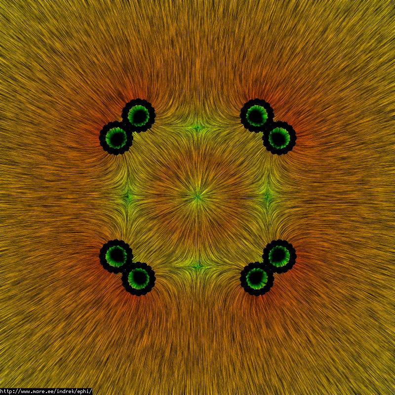
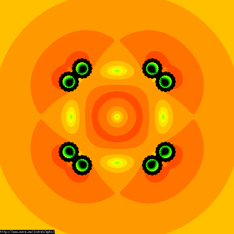
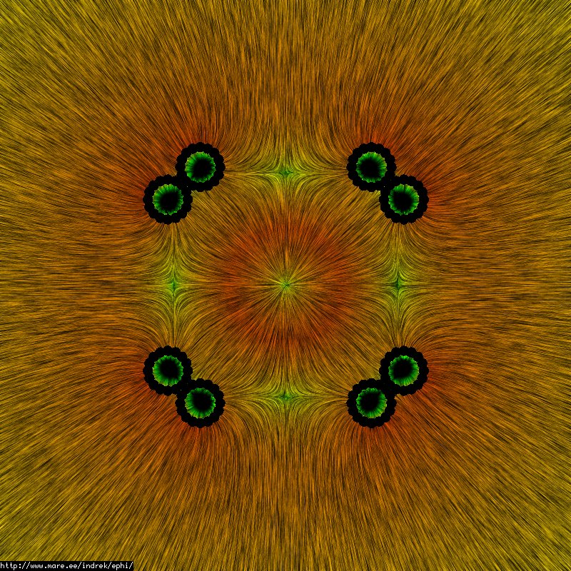
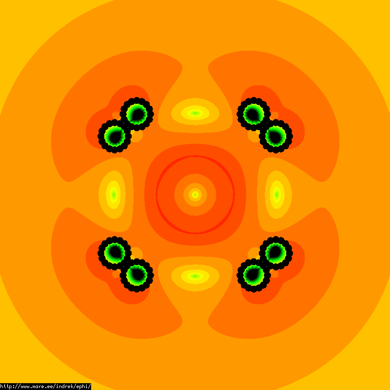
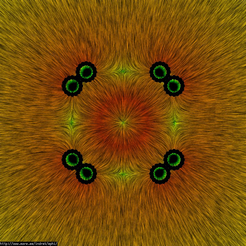
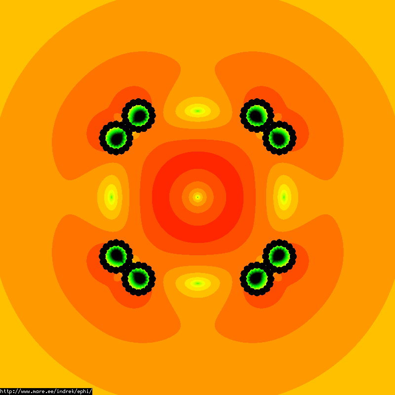
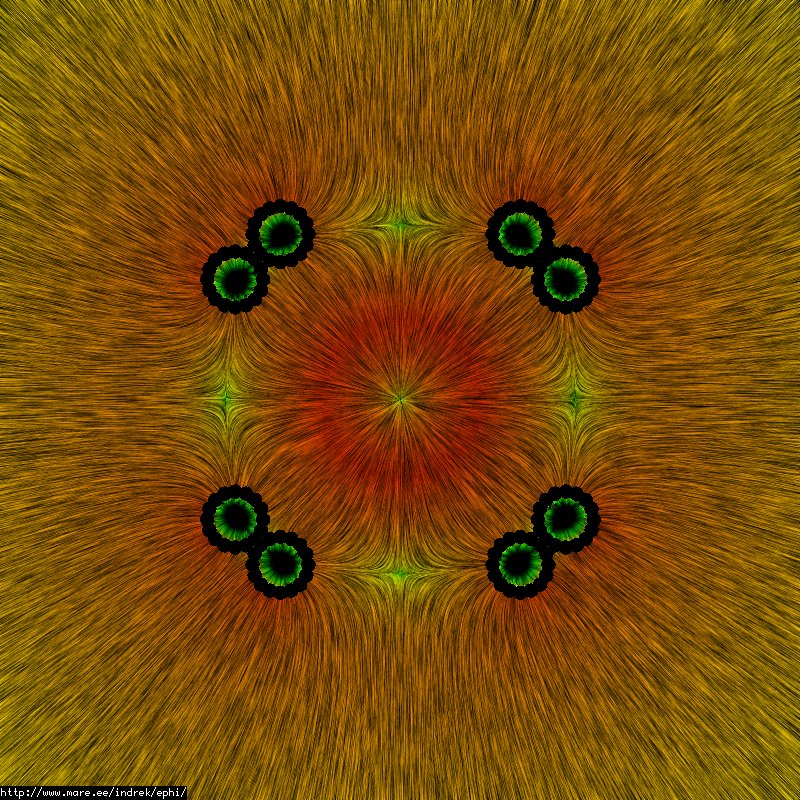
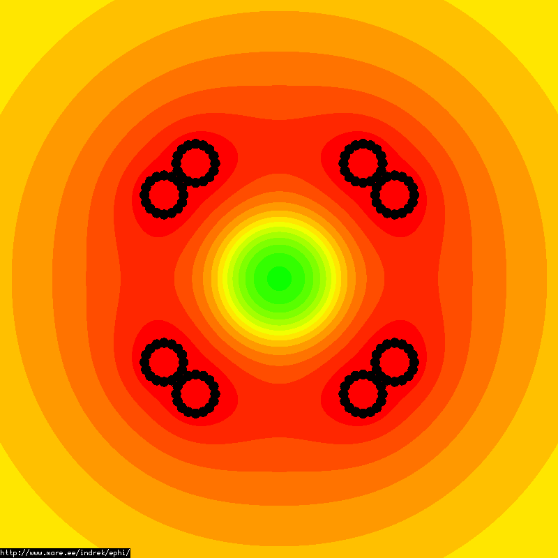
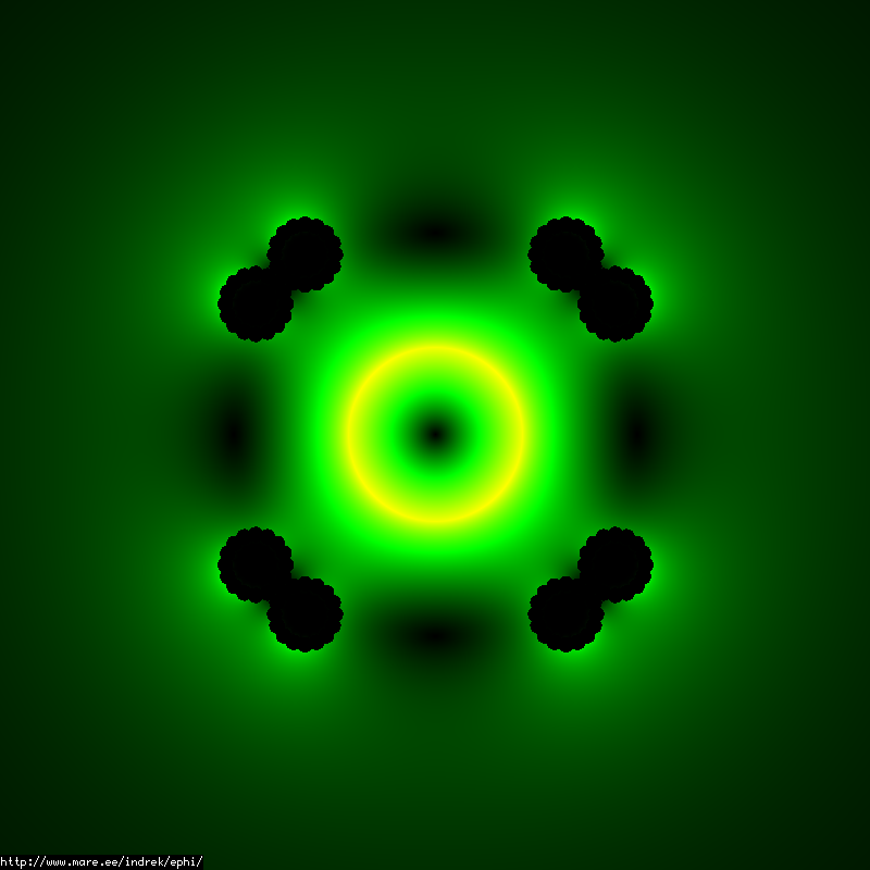
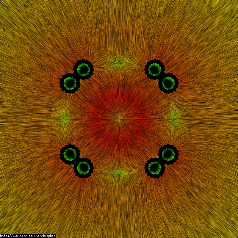
And now it's time for this page's useful information. Lets put a 0.1m radius sphere of uniformly distributed charge within the middle of the system and see what kind of potential wells, capacitances, charges, etc. are involved. The electric potential and electric field of a sphere of uniform charge are calculated like this:
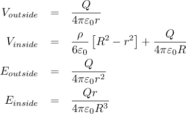
We sample the configuration at various space charge levels and see what happens to the fields and the potential well. If you look at the equations you can see that outside the radius of the sphere the field behaves as if a point charge located in the middle of the sphere. Field levels on different pictures can be compared and you can click on the images to get a bigger picture. Note also that the potential difference between levels in the pictures is around 88V.