In our last experiments I modeled the electric potential and the electric field through point charges on the surfaces and used linear relations/systems to calculate the exact charge at each point. Lets try something more complicated.
I have derived equations for the electric potential and field of a line of charge with variable linear charge distribution. Lets describe the surface as points of charge density and lines between them. If we look closely at the equations we can see that we can similarily derive a system of linear equations against arbitrary potential points:
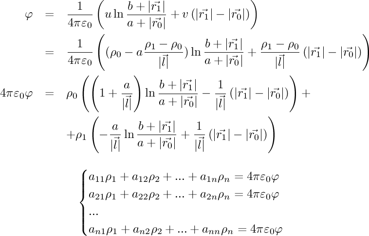
This may look like some fancy math but it's really trivial stuff. Lets see how this works with a torus.
This torus consists of 3696 points and 3696 line segments. The green balls are the reference potential points, they lie directly behind the connecting charge density points between the lines. The estimated capacitance is 31.102pF. This is a bit off from the expected 31.107pF. The reason for the error can be found in two places: the linear distribution of charge in the lines does not reflect reality that well and secondly the lines clip the surface of the torus, reducing its size. If I increase the resolution of the calculations I will get values closer to the expected. The visualized electric field though shows a smoother image than compared with point charges. The area where the field is zero within the torus is more circular.
All in all the form of the math is not that much different from the system of point charges we looked into before. So qualitatively we don't get much better results. The field values are slightly smoother and look better but this comes with a penalty in calculation complexity. Then again this method might be more interesting in analyzing more complex conductor shapes.
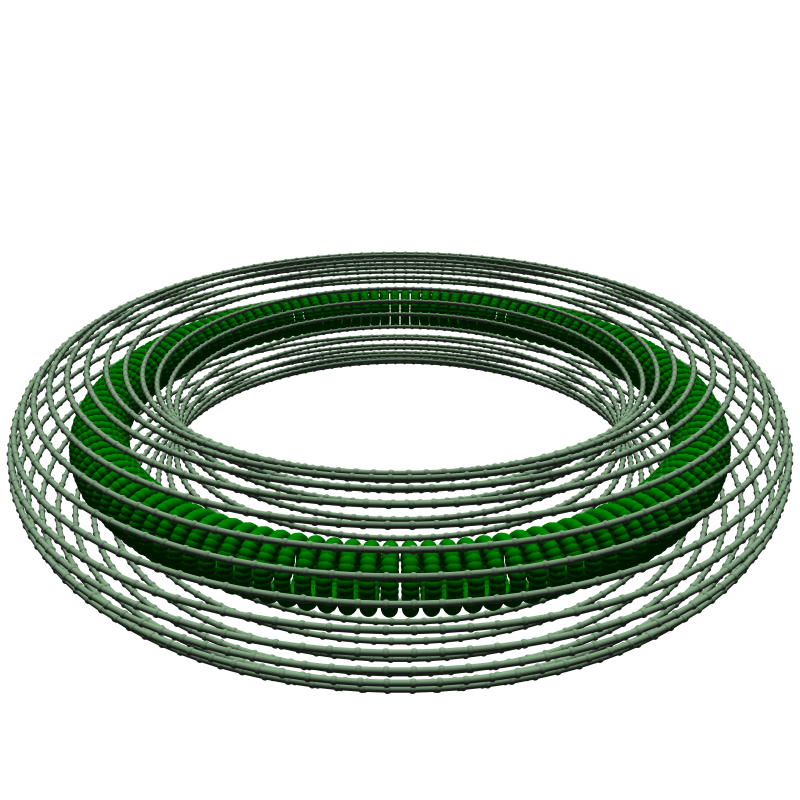
In part II I ran a series of simulations to show the electric field within the cube polywell with various space charges present. Lets run the same experiments but this time analyze the numbers produced themselves. How do the charges relate to themselves and the potential well?
This time I set the same system, R=0.15m coil radius, 0.07m coil thickness, 0.01m spacing. But with coil voltage of 10,000V and potential well down to 13207V. The data produced:
| CSV: | polyp.csv |
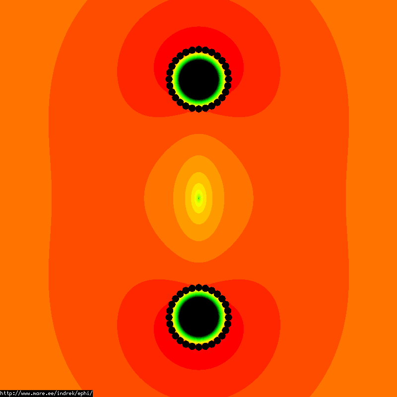
Lets look how the charge on the coils grows as the space charge grows. The
growth is linear and seems to match with the space charge added.
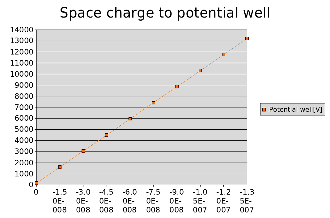
What about the space charge to the potential well formed? The growth here again is linear. But don't forget the charge in the middle is modeled as a uniform sphere of charge and so is not the real thing.
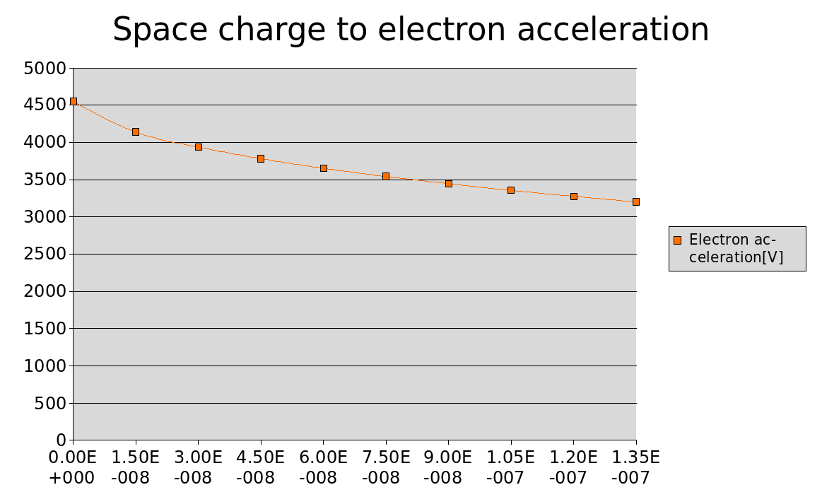
Lets put the electron guns at fixed 2*R=30cm from the coil face and assume the electrons have initial speed of 0eV. Lets measure the accelerating potential difference as the electrons are attracted towards the system. It seems the acceleration drops with increased space charge. Note again that in a real polywell some of the charge would be flowing back through the cusps reducing the acceleration of new electrons even more. There is one more observation we can make. At the distance of 2*R the acceleration is around 4000 volts. But if the well depth is well into 13000 volts - how can the electrons reach the middle of the system? The answer is that they can't. What does that imply? My guess is that the ball of electrons in the system just keeps growing and ballooning and you can't really get a deeper well than the speed of electrons you put in.
There is one flaw with the electron guns and this analysis. They are supposed to be at ground potential. That will change the picture significantly.
Copyright © 2007 Indrek Mandre